Notes on Nonlinear Dispersive Wave Equations Workshop in Oberwolfach

James Colliander

2010-10-04 86 min read conference

This page contains notes by J. Colliander taken at the workshop:

$MFO$

Nonlinear Waves and Dispersive Equations
Organizers:
Date: September 12th - September 18th, 2010

I apologize for any mistakes! If any of the speakers would like me to post (or link to) their slides, please send me the file. –Jim Colliander

Jérémie Szeftel: Alas, I missed this talk….thanks Air Canada.
1. arXiv
2. slides
Sebastian Herr: Small data theory for energy critical periodic NLS
1. Warm-up remarks
2. $N L S \pm 5 (T 3)$
3. New Strichartz Estimates
4. Perturbative Analysis
5. Trilinear Strichartz
6. Sketch of proof
7. Contraction estimate
8. Remarks
9. Questions
Benjamin Schlein: Effective evolution equations from many body quantum dynamics
1. Introduction
2. Boson Stars
3. Dynamics of Bose-Einstein Condensates
Adrian Constantin: Camassa-Holm
1. Physical Background
2. Emergence of Camassa-Holm Equation
3. Geometric viewpoint as a geodeisc on the diffeomorphism group
4. Integrable Sturcture
Claudio Muñoz: Dynamics of gKdV solitons under perturbations by potentials in front of nonlinear term
Mihalis Dafermos: Superradiance, trapping and decay for waves on Kerr spactimes in the general subextremal case $| a | < M$ .
1. Boundedness and decay for $◻ g ψ = 0$ on Schwarzschild and Kerr
2. Current state of the art for the quantitative study of $◻ g ψ = 0$
3. Review of the main features of Kerr Spacetimes
4. Proof of integrated local energy decay.
5. Open Problems
Stephen Gustafson: Dynamics on near-harmonic Schrödinger and Landau-Lifschitz maps
1. Regurlarity vs. Singularity: energy critical problems
2. Equivariant Maps
3. New results: global solutions for degree 2 (LL) with $a 1 > 0$ .
4. Standard “modulation theory” approach
5. A remedy for $m \leq 3$ and its cost.
6. Conclusions
Ioan Bejenaru: Near soliton evolution in 2d Schrödinger Maps
1. Large Data Theory
2. Equivariant Harmonic Maps on $S 2$ .
3. Basic setup for stability/instability
4. Modulation Theory
Frank Merle: Isolatedness of characteristic points for blow-up solutions of semilinar wave equation
1. Semilinear Wave Equation, Blowup Surface
2. Summary of Results
Ben Dodson: Defocusing $L 2$ -Critical NLS
1. Mass-Critical NLS
2. Minimal Mass Blowup Solution Strategy
3. Galilean Invariance Observations
4. $L 2 t$ interval decomposition induction argument
5. Decomposition of nonlinearity
6. Questions
7. Postlude
Killip: Energy Supercritical Wave Equation in 3d
1. Introduction
2. Step 1: Minimal Criminal
3. Step 2: Minimal Criminal satisfies one of three scenarios:
4. Step 3. No finite time blowup solutions.
5. Step 4. Solutions move more slowly than light speed.
6. Step 5. $L p$ decay.
7. Step 6. A more quantitative $L p$ estimate.
8. Step 7. Climax $E (u) < \infty .$
9. Step 8. Completion of Theorem
10. Questions/Comments:
Wilhelm Schlag: Global dynamics above the ground state energy
1. Klein-Gordon and Schrödinger Equations
2. Questions and Answers
3. Computer Simulations
4. Structures in Phase Space
5. Final State Descriptions near $Q$
Jeremy Marzuola: Scattering and soliton stability in $˙ H - 1 / 6$ for quartic KdV
1. The problem
2. Previous Results
3. Function Spaces
4. Steps of Proof
5. Energy spaces
6. Nonlinear Modulation
7. Postlude
Sijue Wu: Global and almost global wellposedness of the two and three dimensional full water wave equations
1. Introduction
2. LWP
3. Global-in-time behavior
4. Statements
5. Normal Forms Discussion
Nickolay Tzvetkov: On random data nonlinear wave equations
1. Framework
2. Randomized data on $T 3$
3. Steps in the proof
4. On the proof of the Global existence step for $s > 0$
5. Questions
Pierre Germain: Global existence for coupled Klein-Gordon equations with different speeds
1. General Problem: Understand global existence and scattering for nonlinear dispersive equations with very nice data.
2. NLW, $d = 3$
3. NLKG
4. Statement
5. Spacetime resonance method
6. Application to our problem
7. Questions
8. Postlude:
Oana Ivanovici: Dispersive Estimates on convex domains
1. Introduction
2. Applications
3. Cusp solutions hugging the boundary
4. Proof
Axel Grünrock: Cauchy Problem for higher order KdV and mKdV equations
1. Equations
2. Earlier Results
3. New Results
4. Questions
5. Postlude
Selberg: Global existence for the Maxwell-Dirac system in two space dimensions
1. Maxwell-Dirac and Dirac-Klein-Gordon
2. Results
3. 2d DKG
4. What lies behind the proof?
Jason Metcalfe: Long time existence for nonlinear wave equations in exterior domains
1. Problem $S$ :
2. Problem $Q$ :
Scipio Cuccagna: The Hamiltonian structure of the nonlinear Schrödinger equation and the asymptotic stability of its ground states
Alexandru Ionescu: Uniquness theorems in general relativity
1. Spacetimes
2. Key properties of Kerr spacetimes:
3. Postlude

Jérémie Szeftel: Alas, I missed this talk….thanks Air Canada. ↩

Sebastian Herr: Small data theory for energy critical periodic NLS ↩

(joint work with Tataru and Tzvetkov)

Energy critical NLS focusing or defocusing on a manifold M. Specific examples with Laplace Beltrami operator. Mostly intersted in manifolds with periodic geodesics. For example $T 3$ or tori crossed with $R d$ .

Target is LWP.

Warm-up remarks ↩

Warm up: $M = R d$ . Strichartz, dual Strichartz, dispersive decay $⟹$ (Cazenave-Weissler) LWP.
Non-Euclidean cases: Asymptotically Euclidean and nontrapping metrics have been studied.
Failure of sharp Strichartz estimates on torus and on sphere.
Trapping creates geometric obstructions to dispersion.
Trapping can create instabilities and failure of Strichartz estimates.
Known estimates: Strichartz with a loss of derivatives.

$N L S \pm 5 (T 3)$ ↩

Available estimates have some loss. The loss obeys the scaling but it is insufficient to control the quintic nonlinearity. We end up needing an $L 4$ estimate, which is unavailable.
Our strategy is to use multilinear, scale invariant versions of Strichartz estimates to better share the derivatives.
Use almost orthogonality wrt spacetime to reduce estimates to smaller scales.
Replacements/refinements of the $X s, 1 / 2$ ? We use the critical function spaces $U p, V p$ .
We will need refinements of these spaces which are sensitive to finer than dyadic frequency localizations.

New Strichartz Estimates ↩

We have the Strichartz estimates on functions supported on cubes in Fourier space
For all rectangular sets of arbitrary orientation and center, we get a better bound!
This boils down to a classical estimate (Landau 24) for counting the number of lattice points on 6d ellipsoid.

Perturbative Analysis ↩

$U p$ : Definition involving all partitions of the line using $U p$ -atoms.
These are Banach spaces which embed into $L \infty$ .
$V p$ : We need another type of space. These are functions of finite $L p$ variation over the partitions of the line.
$U p \to V p r c \to L \infty$ (Embeddings)
$‖ u ‖ U p Δ H s = ‖ e - i t Δ u ‖ U p (R; H s)$ . (Similarly wrt $V p$ , as in Ginibre’s Asterisque.)
We choose then $p = 2$ and call the resulting spaces $X s$ and $Y s$ .
Properties: $U 2 Δ H s \to X s \to Y s \to V 2 Δ H s$ (Embeddings)
We define restrictions to smaller time intervals….
$X s$ and $Y - s$ have a nice duality relationship.

Trilinear Strichartz ↩

Refinement which generalizes Bourgain’s $p = 6$ Strichartz estimate.

Sketch of proof ↩

Decompose the largest frequency $N 1$ annulus in cubes of the second largest frequency $N 2$ .
We can replace $Y 0$ by $V 2 Δ L 2$ .
We deduce control on the quintic nonlinearity using the trilinear estimate. Some gain is obtained by playing with the exponent $p$ in the $U p$ spaces, which he attributed to elementary properties of these atomic spaces.
This gain and some other slack in the other trilinear estimate allows one to sum up over the dyadic scales.

I am confused at this point? Do we have some derivative slack or are thing really tight? Since we are considering an

H 1

critical problem, there can be no slack….I discussed this with Sebastian a bit after the talk. I was confused; there is no derivative slack.

Next, there is a new localization (the rectangle decomposition). The cubes are decomposed into almost disjoint strips of a certain width. The almost orthogonality is gained from the temporal frequency! (This reminded me of the ideas from Koch-Tzvetkov and later developed by Ionescu-Kenig)

Contraction estimate ↩

It is not necessary to use the rectangles to get this estimate. For the qunitic case, we can avoid the rectangles. For the cubic NLS, by duality you have a 4-linear estimate and by Cauchy-Schwarz you are reduced to bilinear estimates. For the cubic case, it is necessary to use the rectangle decomposition.

Remarks ↩

With similar ideas, they can treat the cubic case on $R 2 \times T 2$ or $R 3 \times T$ .
This involves bilinear refinements instead of cubic refinements.
small data GWP for energy critical NLS on certain manifolds where arguments of the Euclidean setting fail.
Large data is a very interesting problem.
This is the first critical result for NLS on a compact manifold.
Quintic NLS on the 3-sphere? Strichartz estimates fail but possible to control second Picard iteration.
Cubic NLS on $T 4$ .

Questions ↩

Flat waveguides?
$L 2$ critical case?

Benjamin Schlein: Effective evolution equations from many body quantum dynamics ↩

Resources: Schlein’s talk at ICMP 2009, Schlein’s Zurich Lectures

Introduction ↩

Consider

N

particles moving in 3d. These particles can be described in quantum mechanics by a wave function

Ψ N \in L 2 (R 3 N)

. The probability density

| Ψ N (x 1, x 2, \dots, x N) | 2

represents the probability of finding particle 1 at location

x 1

and so forth. Bosons are symmetric wrt particle interchange. Fermions are antisymmetric. We will restrict in this talk to Bosonic symmetry: For all permutations

π

Ψ n (x π 1, \dots, x π N) = Ψ (x 1, \dots, x n)

The dynamics of the wave equation is governed by the Schrödinger equation $i \partial t Ψ N = H N Ψ N$ Typically, $H = N \sum j = 1 (- Δ x j + V e x t (x j)) + λ N \sum V (x i - x j) .$ We have well-defined local dynamics. The problem is that we have way too many particles in typical physical systems. We want to find effective descriptions of the dynamics. In certain regimes, we can approximate this complicated but linear evolution using effective equations

Mean Field Regime

The particles interact with many other particles. The strength of each of these many interactions is small so that the effect of all of them is of order 1:

N ≫ 1, λ ≪ 1

. We will assume that

N λ \sim 1

. The dynamcis generated by the mean field Hamiltonian:

H m f = \sum (- Δ x j + V e x t (x j)) + κ N N \sum V (x i - x j) .

We study the dynamics emerging from a product wave function:

Ψ N (x 1, \dots, x N) = N \prod j = 1 ϕ (x j)

Because of the interactions, we can’t expect that the product wave function remains of product form. But, in the mean field case, we might expect that

Ψ N (t) \sim ϕ (t) N

. If we assume this, we obtain a self-consistent Hartree equation. Here is the heuristic step:

κ N N \sum V (x i - x j) \sim κ N i \neq j \sum \int V (x i - y) | ϕ (y) | 2 d y \sim κ (V * | ϕ (t) | 2) (x j) .

Reduced Densities

$γ N (t) = | ψ N (t) ⟩ ⟨ ψ N (t) |$
Partial traces
- When we take partial traces, we lose some information. It is integrated out. However, we are only interested in the data that can be extracted based on measurements of finitely many particles.

Theorem: (Under suitable assumptions on

V

). Let

ϕ \in H 1 (R 3), Ψ

a pure product wave function,

Ψ N (t)

the linear evolution of the many body system. The for all fixed

k \in N, t \in R

, the reduced density matrices converge to the projectors build on the

ϕ

evolutions where

ϕ

solves the Hartree equation.

The more singular the potential, the more difficult it is to prove the theorem.
Spohn 1980: proved this for bounded $V$ .
Erdös, Yau 2000: $V (x) = \pm 1 | x |$ .
Rodnianski, Schlein 2008: , gives quantitative convergence with control by .
- The RS work was based on an approach by K. Hepp.
- The approach is based on a representation of the problem on Fock space.
- Coherent states and quantum field theory ideas.
Knowles, Pickl 2009: Improved to more singular potentials.
Grillakis, Machedon, Margetis 2009 I, II: Second order corrections to the mean field dynamics, giving norm convergence.

Boson Stars ↩

$N$ particle Hamiltonian $H = N \sum \sqrt 1 - Δ x j - G \sum 1 | x i - x j |$
$N ≫ 1, G ≪ 1, N G = κ$
(kappa critical) such that:
- $inf ⟨ Ψ, H N Ψ ⟩ ‖ Ψ ‖ 22 = 0 i f κ \leq κ (N)$
- $inf ⟨ Ψ, H N Ψ ‖ Ψ ‖ 2 = - \infty i f κ \geq κ (N)$
- Lieb, Yau proved that $κ (N) \to κ H$ as $N \to \infty$
Look at the corresponding effective field equation.
- For $κ \leq κ H$ , we have global well-posedness.
- For $κ \geq κ H$ , there exists finite time blowup solutions (Fröhlich-Lenzmann 2006).

Theorem (Michelangeli-Schein 2010): Let

ϕ \in H 2 (R 3)

and form product wave function

Ψ N

and let

Ψ N (t)

evolves according to the regularized Hamiltonain (where the singularity is tamed by adding a small positive term to denominator which vanishes as

N \to \infty

). If we have

H 1 / 2

control on the nonlinear level by constant

k

over a time interval

[0, T]

then we have convergence. Moreover, if the nonlinear problem explodes then the energy per particle in the linear problem also blows up. (Hypotheses were a bit strange to me….I asked about it after the talk and need to look at the paper.)

Dynamics of Bose-Einstein Condensates ↩

Drop the external potential. Effective dynamics in this case is described by the Gross-Pitaevskii equation:

N L S + 3

The derivation of effective dynamics in this setting has only been established for the defocusing case.

Adrian Constantin: Camassa-Holm ↩

Physical Background ↩

2d water waves over a flat bed. He draws a curve above a flat bottom at

y = - h 0

and the free surface is given by the graph

y = η (x, t)

. He writes the Euler equations, mass conservation, imposes reasonable boundary conditions. These are generally accepted to be the right model. I will work with one other assumption:

u y - v x = 0

: irrotational. There are various scales you can plug into the problem and then you can non-dimensionalize. The problem can then be written in terms of just two parameters

ϵ

and

δ 2

where:

ϵ = 2 h 0,

δ = h 0 λ

Small amplitudes

ϵ ≪ 0

and

δ

is the shallowness parameter so shallow water wave theory means that

δ

small. Shallow water small amplitude is when

δ ≪ 1

and

ϵ = O (δ 2)

. If you study this, you get KdV and BBM equations. In this regime, these model equations enjoy global existence. The nondimensional form of the KdV equation is

η t + η x + 3 ϵ 2 η η x + δ 2 6 η x x x = 0.

Here is the emerging BBM:

η t + η x + 3 ϵ 2 η η x + δ 2 (β + 16) η x x x - β δ 2 η x x t = 0, β \geq 0.

KdV is completely integrable and has solitons. BBM has some nice analytic features but only 5 conserved quantities. These derivations are

O (δ 4)

Where does Camassa-Holm come into this business? Since all the waves that are physically reasonable, we have global existence. We would like to have a simple model that captures the phenomenon of wave breaking: $η$ is bounded, $| η x |$ becomes unbounded in finite time. (This is described as a desirable extension in the book Linear and Nonlinear Waves, by Whitham.)

Emergence of Camassa-Holm Equation ↩

Moderate amplitude (shallow water):

ϵ = O (δ), δ ≪ 1.

Johnson found a path like this to see Camassa-Holm emerge. (“Unfortunately, the original derivation of that equation was not correct.” “They assume that $ϵ$ is small and later they assume that $1 / ϵ$ is small…”) You can derive an equation for the horizontal velocity at a particular depth. If you do this derivation at depth $1 \sqrt 2 | h 0 |$ . Another equation called Degasperi-Procesi emerges when you consider this at a different depth: $u t - u t x x + 3 k u x + 4 u u x = 3 u x u x x + u u x x x$ Both of these equations are integrable! (I did not know about the D-P equation before…) Both of these equations have solution which break down, in the fashion of wave breaking described above.

For CH, we have some conservation laws which implies the solution stays in $L \infty$ . Fokas and Fuchsteinner found the CH equation in a list of 12 equations that are the only completely integrable equations. It is difficult to use the integrable systems machinery to study the wave breaking. For DP, if you start with data in a nice enough space (say $H 3 / 2$ ) and you can then prove the solution stays in $L \infty$ .

Tzvetkov Q: Can the solution be extended after the wave breaks? A: You might be able to extend the solution like shocks. But the relevance of the wave breaking event in CH, it is not clear whether the CH is a good approximation of the Euler equations. Therefore, even if the PDE theory for CH can be extended, this does not mean you have a relevant extension modeling the water wave problem.

Geometric viewpoint as a geodeisc on the diffeomorphism group ↩

There is this famous paper of Arnold that shows that Euler may be viewed as a geodesic flow on the diffeomorphism group. CH and KdV can be similarly interpreted as a geodesic flow on the Bott-Virasoro algebra. This geometry thing is very nice, very appealing. However, this geometric point of view does not give a useful consequence from the viewpoint of analysis.

The best result for CH is that when the solution does not change sign it stays global. This is built from Nöther’s theorem, which provides a different view on the CH equation

Write $D = [ϕ : C \infty o r i e n t a t i o n p r e s e r v i n g d i f f e o s]$ . This is a Lie group and the tangent space at the identity is $C \infty (S)$ . We can then move this tangent plane around using Lie algebra properties by right-translating. The geodesic equation looks like $ϕ t = u (t, ϕ)$ where $u \in D$ .

If I do this for $L 2$ , I get $u t + 3 u u x = 0$ . However, the Riemannian exponential map $e x p R$ is not a local chart.
If I do this for $H 1$ ( I believe this is referencing the Riemannian structure imposed on $C \infty$ diffeos) we get CH.
Consider the Bott-Virasoro Algebra $V i r = C \infty \times R$ and you do some Bott cycle thing which looks like a diffeo flow with a twist, you get KdV. (This is a result of Olsheyenko(?) and Khesin.)
DP equation also has some interpretation this way but it is more complicated.

Integrable Sturcture ↩

CH Lax Pair. This is an isospectral problem. For CH, we have $ψ x x = 14 ψ - λ m ψ, m = u - u x x + k$ . This is a weighted spectral problem. If $u$ solves CH, then the eigenvalues of this equation are time independent.
DP Lax Pair. $ψ x x x - ψ x - m z 3 ψ = 0, z \in C, m = u - u x + k$ . When $m$ is strictly positive, we can perform certain Liouville substitutions which allow us to recast this as a regular Sturm-Liouville problem.

This talk did not properly survey the literature. Instead, the talk was intended to highlight a physically relevant derivation of the CH and to show that this equation is mathematically and physically interesting.

Tzvetkov asks: Is there a Miura transformation? Seems to be no….although AC appeared to me to answer a different question.

Merle asks: Can you track the blowup using the integrable machinery here? We need estimates on the eigenvalues hold if $m > 0$ and you can give examples which show that sign-changing $m$ breaks down the needed estimates on the eigenvalues.

Ponce asks: What is the best LWP theory for CH? Answer: Kato’s theory needs $H 3 / 2$ . You have existence, uniqueness and continuous dependence in $H 1$ , but the continous dependence is weaker.

Ponce asks: Is the peakon stable? A: Yes, this is a result of Molinet and El Dika.

Claudio Muñoz: Dynamics of gKdV solitons under perturbations by potentials in front of nonlinear term ↩

My computer ran out of battery….

arXiv: Muñoz on KdV

arXiv: Muñoz on NLS

Mihalis Dafermos: Superradiance, trapping and decay for waves on Kerr spactimes in the general subextremal case $| a | < M$ . ↩

(joint work with Igor Rodnianski)

Kerr family $(0 \leq | a | \leq M)$ of metrics (in Boyer-Lindquist coordinates) $g M, a = - Δ ρ 2 (d t - a sin 2 θ d ϕ) 2 + ρ 2 Δ d r 2 + ρ 2 d θ 2 + sin 2 θ ρ 2 (a d t - (r 2 + a 2) d ϕ) 2 .$ Here $ρ 2 = r 2 + a 2 cos 2 θ, Δ = r 2 - 2 M r + a 2 = (r - r -) (r - r +), r + \geq r - .$ This is a vacuum solution $(R μ ν = 0)$ and has Killing fields $\partial t, \partial ϕ$ . The domain of outer communications is $r > r +$ . The case $a = 0$ is Schwarzschild 1916. The Kerr case is $a \neq 0$ and was discovered in 1963.

Penrose diagram for Kerr $(0 < | a | N M)$ . What is a black hole? A spacetime has a black hole if the past of this infinity is not the entire spacetime. Both Kerr and Schwarzschild are expected to be unstable and the structure of the singularity should be something in between.

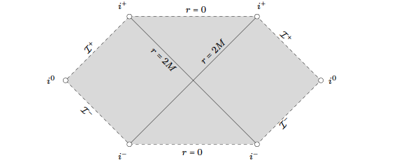
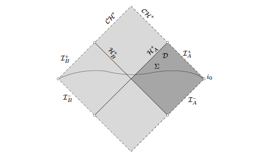
Penrose Diagrams (images taken from Dafermos-Rodnianski)

Penrose diagram of Schwarzschild spacetime

$Penrose diagram of Schwarzschild spacetime$

Penrose diagram of Kerr spacetime

$Penrose diagram of Kerr spacetime$

Boundedness and decay for $◻ g ψ = 0$ on Schwarzschild and Kerr ↩

These are natural questions from several points of view. One important application of these ideas is to address the stability properties of these solutions of the Einstein equations.

Current state of the art for the quantitative study of $◻ g ψ = 0$ ↩

Boundedness in general class of $C 1$ stationay axisymmetric spacetimes [DR].
“Integrated local energy decay” for exactly Kerr:
1. Slowly Rotating Case $| a | ≪ M$ [DR], Tataru-Tohaneanu, Andersson-Blue
2. $| a | < M$ , [DR] this talk!.
Pointwise-in-time decay from 1. and 2. (energy based method [DR] based on resolvent method of Tataru)

We typically think of proving decay as a two step process. We first prove that some spacetime integral of energy to the future an arbitrary hyperboloidal space-like hypersurface controlled by the energy on the hypersurface. This type of result has been shown in the slowly rotating case. Once we have items 1. and 2. (boundedness and integrated local energy decay) we can use the vector field method to get pointwise-in-time decay. These methods appear to be robust and might be applicable to nonlinear problems.

Review of the main features of Kerr Spacetimes ↩

Red-shift (associated to the event horizon)
Superradiance
Trapping (trapped null geodesics)

Red-shift

Two observes move in spacetime. You think of observer A emitting constant frequency signals and you imagine these being received by observer B so the frequency is shifted to the red. First discussed in 1939 by Oppenheimer-Snyder. Extremal case

a = M

: The red-shift factor at the horizon vanishes. The positivity of the surface gravity is a geometrical object underlying the red shift.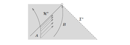

$Penrose diagram of Red Shift$

Superradiance

In Schwarzshild, the killing v.f.

\partial t

is timelike n the exterior becoming null on the horizon. Thus there is a conserved (by Nöther) non-negative definite energy by the time-like condition. The only subtlety is that the energy degenerates at the horizon.

In stationary perturbations of Schwarzschild, $\partial t$ in general becomes spacelike near the horizon. this happens already for Kerr with $0 \neq | a | ≪ M$ . The corresponding energy is conserved but does not have a sign. For particle motion, this leads to the so-called Penrose Process. For waves, this leads to the phenomenon of superradiance (Zel’dovich).

In particular, using the conservation law associated to $\partial t$ one cannot prove a priori boundedness, even away from the horizon. The energy radiated to null infinity might be bigger than the initial energy and this is called Superradiance.

For Schwarzschild, the only trouble is near the horizon because we have a useful energy control for radiated energy to null infinity. For Kerr, we don’t have that because of the superradiance phenomenon and this creates new difficulties. We need to prove boundedness and decay everywhere, not just near the horizon.

Trapping

On Schwarzschild, the photon sphere

r = 3 M

has the property that it contains null geodesics. These null geodesics thus neither escape to null infinity nor to the horizon. In Kerr, the behaviour persists, but it is more complicated! It is not obviously located in physical space but can be thought of more easily inside phase space. One can concentrate energy for arbitrarily large times near trapped null geodesics. One has to capture this to prove dispersive results. In particular, pointwise-in-time decay estimates for energy must lose derivatives (Ralston).

Proof of integrated local energy decay. ↩

We will only discuss the first energy. Higher order estimates require commutation with the redshift vector field, the Hawking v.f. and

\partial t

The method of proof will exploit energy currents.

In the large $a$ case, the construction of these currents will need to frequency localized for two reasons.

To distinguish between non-superradiant and superradiant frequencies.
To degenerate at the correct value of r.

A convenient way of doing both at the same time is frequency localizing via Carter’s celebrated separation of the wave equation. Kerr geometry only has two killing fields. This is not enough to separate the equation. However, there is some extra symmetry there that helps you. In view of Ricci flatness, this separability is equivalent to separability of Hamilton-Jacobi equations and the existence of a Killing tensor. These three objects are devices to extract this hidden structure.

Separation.

Big display….can’t keep up with that. We are studying

◻ g ψ = F

(where

F

arises from cutoffs) and we take

ˆ Ψ

and rewrite it using some structure of an oblate spheroidal metric in the

θ, ϕ

variables. The content of what Carter noticed is that when you do this, you can show that there is a hidden ODE lurking in this decomposition…..

More big display…working pretty hard here, lots of indices….new coordinate $r *$ so that things look more like the Regge-Wheeler coordinates in Schwarzschild. With this decomposition, we can identify the superradiant frequencies. The superradiant modes should be thought of as the modes which send infinite negative energy through the horizon.

Completely separated energy current identies (analogues of $\nabla μ (T μ ν (ψ) (y \partial r *) ν)$ , etc.)

Lots of notation with symbols I don’t know how to make….

General Idea

From the above currents, produce integral identities with positive definite underlined bulk terms and (upon summation) we get the integrated decay except in regions which can’t be handled this way, basically because these frequency ranges are associated with trapping.

Kerr for small $| a |$ . The constructions for all the other frequency ranges can be easily perturbed to yield positive definite bulks. The boundar terms, however, are not a priori controlled, this is the problem of superradiance. Since $| a |$ is small, this can be remedied by adding on a small amount of the redshift identity. Basically, for the small $| a |$ case, we have very little superradiance and can control it with the red shift. For large $| a |$ , we need another idea.

The key observation seems to be that superradiant frequencies are not trapped. You can accomodate the superradiance using this idea by using the red shift.

Remark 1: In the small rotation case, the relationship between superradiance and red shift was the key idea. Remark 2: There are no trapped null geodesics which are orthogonal to $\partial t$ . This is a phenomenon identified by Alexakis-Ionescu-Klainerman in their works on uniqueness properties.

Some other important results

Positive and negative cosmological case
Ohter equations, like Dirac, Maxwell instead of wave equation. (Blue, Hafner, Finster et. al)

Open Problems ↩

Extremal case $a = M$ (recent results of S. Aretakis)
Higher dimensions (Schlue, Laul-Metcalfe)
Other measures of decay, Strichartz, …
Robust additional decay
Maxwell equations on Kerr (Blue) (Earlier work by Blue on Schwarzschild)
Equations of gravitational perturbation
Nonlinear stability of Kerr?

Stephen Gustafson: Dynamics on near-harmonic Schrödinger and Landau-Lifschitz maps ↩

(w. Nakanishi, Tsai) The paper that precedes the new stuff here is posted.

Landau-Lifschitz (30s), magnetizations $u (t, x) \in R 3$ with a constraint $|u(t,x)| = constant. The Landau-Lifschitz equation is:

$u t = a 2 u \times Δ u - a 1 u \times (u \times Δ u), a 1 \geq 0.$

Broader context:

$u (\cdot, t) : R 2 \to S 2 .$
energy $E (u) = 12 \int R 2 | \nabla u | 2 d x$
heat flow $u t = Δ u + | \nabla u | 2 u = - E' (u)$
Schrödinger Map: $u t = u \times Δ u = J E' (u)$ , $J$ is a complex structure.
Landau-Lifschitz is a combination of these equations
Also related to wave maps

Regurlarity vs. Singularity: energy critical problems ↩

Energy is scale invariant in

R 2

E = \int R 2 | \nabla u | 2 \geq 4 π | d e g r e e (u) |

iff Harmonic map. So, what can you say?

Heat flow:

$E < 4 π ⟹$ global smooth solutions Struwe 1985.
$E > 4 π ⟹$ singularities may form, follows from Chang-Ding-Ye 92 via subsolution construction.

Wave map:

$E < 4 π ⟹$ global smooth solutions Sterbenz-Tataru 09
$E > 4 π ⟹$ singularities may form, follows from Chang-Ding-Ye 92 via subsolution construction. Rodnianski-Sterbenz 06, Kreiger-Schalg-Tataru 08, Raphael-Rodnianski 09

Schrödinger Map:

$E$ small $⟹$ global Bejenaru-Ionescu-Kenig-Tataru 08
Open: larger energy, singularity, for LL also.

Equivariant Maps ↩

Simples setting: near harmonic, equivariant maps.

$m \in Z +$ is the degree
$(r, θ)$ are polar coordinates
$R = ˆ k \times$ (rotation about $ˆ k$ )

2-parameter family of harmonic maps (at minimal

E = 4 π m

). The energy is constrained. We work in a small energy shell above the

4 π m

level. This is a restrictive class but known blowups are in this class. For heat flow case, we only have blowups with

m = 1

but for wave maps we have examples with

m \geq 1

Theorem Gustafson-Nakanishi-Tsai 09: For $m \geq 3$ , solutions are global and converge to a (nearby) harmonic map (asymptotic stability):

$$ { {| u(t) - H^{\mu} |{L^\infty}} } + { { { {a1}} E (u(t) - H^\mu) \rightarrow 0 ~(t \rightarrow \infty). $$

Remarks:

includes the pure Schrödinger map case $a 1 = 0$
also for heat flow () in a symmetry sub-class:
- solutions are global and converge to a harmonic map family
- the parameters can drift, eg to give infinite-time blowup: $s (t) \to 0$ . In particular asymptotic stability fails. (Here $s$ is the length scale of the harmonic map.)

He draws a picture. A

δ

neighborhood of the harmonic maps in the energy space, viewed as an infinite graph over

s > 0

. For

m \geq 3

, solutions in the

δ

neigborhood move dynamically back down to the harmonic maps. For

m = 2

, you can drift all over the place in the case of heat flow.

New results: global solutions for degree 2 (LL) with $a 1 > 0$ . ↩

Setting, as above with dissipations.

Theorem GNT: For $m = 2$ , solutions are global and converge to the harmonic map family, but not to one particular harmonic map.

The harmonic map family parameter $μ (t)$ does not have to converge in general. But it will converge if the initial perturbation has a slightly faster spatial decay: $u x 1 - u \times u x 2 \in | x | L 1 ⟹ μ (t) \to μ \infty .$
For $m = 1$ and only for the heat-flow, finite time blowup can occur but not for more localized perturbations.

(We expect this holds for (LL) but we have no proof.)

Remark: New results of Bejenearu-Tataru for $m = 1$ Schrödinger map of degree 1. Harmonic mapps are unstable, stable with more localization. You should think of the $m = 1$ Schrödinger map case as the most delicate.

Standard “modulation theory” approach ↩

Take your solution and split it into the harmonic map piece plus a remainder. Rewrite things for this remainder term. You look at the linear part of this equation driving the remainder dynamics. Because of invariances of the equation, the linearized operator has zero modes. What would you do to kill the kernel? Choose the parameter at time

t

so that the perturbation is orthogonal to the kernel of the linearized operator. This leads to an ODE on the parameter dynamics. It remains to get dispersive/diffusive estimates to prove that the parameter converges as time goes to infinity. Do we have these estimates?

Dispersive/diffusive estimates

The remainder

z

is controlled by a derived quantity

q

, so the analysis is a bit indirect and we now fight to control this related quantity. The

L 2

norm of

q

measures the energy gap above

4 π m

. The (recast) remainder

q

satisfies a reasonable nonlinear Schrödinger-(heat) equation. This equation has a potential which depends upon

m

. For

m > 1

, we have a lower bound estimate on the potential

V

. In this case, we can get “Strichartz” estimates on

q

For $m \geq 4$ , this standard approach works G-Kang-Tsai 08, [Guan-G-Tsai 08].
For $m \leq 3$ , the orthogonality condition is incompatible with the desired $L 2 t$ -decay estimates and the standard approach fails.
For $m \leq 2$ ,, the orthogonality condition makes no sense.
For $m = 1$ , we don’t even have an $L 2$ -eigenfuction but rather a resonance.

A remedy for $m \leq 3$ and its cost. ↩

Change the orthogoanlity condition. Instead of demanding that the remainder be orthogonal to the kernel of the linearized operator, you require that the remainder be orthogonal to a localized function (unrelated to the kernel). Of course, there is a penalty for this change. The parameter dynamics ODE transforms then to involve another term and we have different parameter dynamics. This extra term is analyzed in some way.
Solution 1: “Normal form” for $m = 3$ . By integrating by parts a few times, we get good control on a modified quantity $[μ (t) - (ψ s / s | q)]$ . We need control on the correction term. For $m \geq 3$ , the correction basically does nothing so things work as before.
Parameter drift for $m = 2$ heat flow. In this case, the “normal form” correction need not be bounded. For the heat-flow case, it is possible to simplify up to converging errors and the nonintegrability of the correction term can be exploited to drive the blowup, blowdown and oscillation properties of the scale parameter $s (t)$ .
Solution 2: Take $a 1 > 0$ and exploit the dissipation “We need to somehow stop pretending that the Schrödinger and heat equations are the same…” In the dissipative case, we can extract some dissipation on the correction term. (Probably, this decay is not available in the Schrödinger case.) There are some factorization tricks where the operator is recast, some Duhamel tricks…and an iteration on dyadic time intervals where the time dynamics of the parameter $μ (t)$ are updated. What emerges is an upper bound by $log t$ on the parameter $μ (t)$ .

Conclusions ↩

Near harmonic dynamics for (LL) for degree $m \geq 3$ .
For $m = 2$ , more complex behavior.
For $m = 1$ , do finite time singularities form? This is only known for the heat-flow.

Ioan Bejenaru: Near soliton evolution in 2d Schrödinger Maps ↩

(joint work with Tataru)

Much of this will be a deja-vu since it overlaps with Gustafson’s talk.

Schrödinger map, Heisenberg model in ferromagnietism or the conservative part of the Landau-Lifschitz equation. Energy Conservation, scale invariance $s c = n / 2$ which is the threshold for the well-posedness theory. The $n = 2$ case is energy critical.

Main Question: Global regularity of smooth solutons?

Sulem-Sulem 86 established existence of local solutions for $s > [n / 2] + 2$ , and this was improved to $s > [n / 2] + 1$ by McGahagan. An “easier” problem is the global regularity for “small” initial data. Chang-Shatah-Uhlenbeck 00, ….Bejenaru-Ionescu-Kenig-Tataru 08 established GWP of the SM for small data in the critical Sobolev space in $n = 2$ .

Small data now resolved. What happens for large data?

Large Data Theory ↩

The dynamics depend upon the target manifold. For the sphere target, the problem is called “focusing” and for the hyperbolic target, the problem is called “defocusing”. This terminology makes good sense for wave maps but is not as explicitly understood in the case of SM.

A key feature in these problems is played by the existence of solitons: $u \times Δ u = 0$ , which are known as harmonic maps. there are no nontrivial finite energy harmonic maps for the hyperbolic target. There are nontrivial harmonic maps with finite energy for the $S 2$ target.

A SM which fails to be regular at one time, bubbles like a HM.

Main Conjecture: In the hyperbolic case, the problem is globally wellposed independent of the size of the data. In the spherical case, solutions emerging from data below $4 π$ will be globally wellposed while the problem with higher energy may develop singularities.

The above conjectre is known for the harmonic map flow Eells-Sampson 64, Struwe 85, Chang-Ding-Ye 92.

Singularity formation for the WM problem. Recent works RS08, KST08, RR10.

There is some progress on more general targets.

Equivariant Harmonic Maps on $S 2$ . ↩

These are maps from the plan into the sphere. Think that the origin is mapped to the south pole. The point at infinity is mapped to the north pole. Think of the image of the positive x axis as a curve connecting the south and north pole. When you move in the domain around wrt theta one time, the curve connecting n and s pole moves around the sphere some number of times. Once you have these maps, you can fatten them up into a two parameter family of maps.

Basic setup for stability/instability ↩

Define the two parameter family of

m

-equivariant harmonic maps. If you have slightly more energy, then you float around the harmonic map family. But do you stay nearby a particular harmonic map or can you float far away? If you move far, the higher derivatives do not stay under control. We want to describe the trajectory of these maps.

Modulation Theory ↩

Linearize near a soliton, study the zero eigenvalue, and these solutions do not disperse. You want to get rid of this eigenvalue. There is room to do that because we have some choice about which soliton you linearize around. This approach has been developed by Gustafson-Kang-Tsai 06 and Gustafson-Nakanishi-Tsai 09. This has been pushed further recently but involves higher degree hypotheses. We have decided to concentrate on the

m = 1

case.

Theorem (Bejenaru-Tataru):

Let $m = 1$ and $γ ≪ 1$ . The for each 1-equivariant initial data $u 0$ satisfying $‖ u 0 - Q (0, 1) 1 ‖ X \leq γ$ , there exists a unique global solution $u$ so that $u - Q (0, 1) 1 \in C (R, X)$ and $‖ u 0 - Q (0, 1) 1 ‖ C (R, X) ≲ γ$ .

There exists a solution

u

with the additional property that

‖ u (0) - Q (α, λ) 1 ‖

…..ack……slide switched I could not keep up. It is an instability result with a large upper bound. It was not clear to me if the assertion was that this big drift really occurs but certainly this is suggested.

Ionescu-Gustafson-Bejenaru conversation: localizations of the perturbations can restore the stability for the heat flow case…

Frank Merle: Isolatedness of characteristic points for blow-up solutions of semilinar wave equation ↩

Background References (Incomplete)

(joint work with Hatem Zaag)

I want to give a talk about a series of works I have done with H. Zaag on the semilinear wave equation.

Semilinear Wave Equation, Blowup Surface ↩

u t t = Δ u + | u | p - 1 u

Here

p > 1

. Let’s collapse to dimension 1. We have initial data

(u 0, u 1) \in H 1 \times L 2

Summary of the results:

Local Existence: We have local existence until a blowup time $[0, T)$ .
Existence of blowup via ODE method. There is a more refined condition due to Levine: If a (not the same as mine) energy is negative then $T < \infty$ .
The blowup phenomenon can be spatially localized. Therefore, as in the book of Alinhac, you can produce a blowup surface. The solution is well defined on all backwards cones behind the blowup surface.
Question: We want to understand the blowup surface. We don’t know anything about it besides that it is 1-Lipschitz.
A point is called non-characteristic on the blowup surface if the surface has smaller than slope 1 at that point so it does not touch the boundary of the light cone. Let us denote the set of characteristic points on the curve by $S$ . The other points on the curve are non-characteristic and the set of such points is called $R$ . Let us denote the blowup curve by $x \to T (x)$ so it is given by a graph $(x, T (x))$ .

Caffarelli-Friedman 85: For $u 0 \geq 0, u 1 \geq 0$ and use monotonicity of the wave flow in 1 dimension to prove that $\partial t u \geq (1 + δ) | \partial x u |$ and you can prove then that no characteristic points don’t exist.

This result is a bit misleading. We tried to prove the nonexistence of characteristic points and could not do it. So, we turned our attention to proving the existence of characteristic points.

Summary of Results ↩

Existence of characteristic points. There exist initial data $(u 0, u 1)$ which has $S$ nonempty.
$S$ is isolated, $R$ is open.
$T (\cdot)$ is $C 1$ on $R$ .
The only way that a characteristic point can arise is like a “hat”. $T'$ from the right and from the left are well defined. (Alinhac has examples for quasilinear equations which can blowup at all points along a line segment of slope 1.) At points $S$ we have $T'$ of slope 1 on the right and slope -1 on the left.
At points along $R$ , the solution is of one sign and points in $S$ are points where the solution changes sign.

Characteristic points are cusps along the graph of

T (\cdot)

A Lyapunov functional (Antonini-Merle).

He shows that the solution extends outside the light cone behind noncharacteristic points. This gives you the $T'$ well-defined (with same value from left and right) at a noncharacteristic point.

The talk was hard for me to type up and explain well….Frank emphasized that the proofs are quite intricate and not presentable in a linear fashion.

Ben Dodson: Defocusing $L 2$ -Critical NLS ↩

References

Mass-Critical NLS ↩

i u t + Δ u = μ | u | 4 / d u, u (0, x) = u 0 (x), x \in R d

We concentrate on the defocusing case where $μ = 1$ . This equation conserves the quantities

$M (u (t)) = \int | u (t, x) | 2 d x$
$E (u (t)) = 12 \int | \nabla u (t, x) | 2 d x + μ d 2 (d + 2) \int | u (t, x) | 2 (d + 2) d d x$

Strichartz Pairs

(p, q) : 2 p = d (12 - 1 q), d \geq 3, p \geq 2.

$$ A(m) = \sup [ { {| u |}{L^{2(d+2)/(d)}} } (R \times R^d): { {| {u0} |}_{L^2}} =M ] $$

Minimal Mass Blowup Solution Strategy ↩

Theorem (Tao-Visan-Zhang 08): If

u (t, x)

is a minimal mass blowup solution on

I

then

\exists x (t), ξ (t) : I \to R d, N (t) : I \to (0, \infty)

and

u (t, x) = 1 (N (t)) d / 2 e i x \cdot ξ (t) Q t (x - x (t) N (t))

where

Q

changes with time but ranges only in a precompact set. For any

η > 0, \exists C (η) < \infty

such that

$\int | x - x (t) | > C (η) N (t) | u (t, x) | 2 d x < η,$

$\int | ξ - ξ (t) | > C (η) N (t) | ˆ u (t, ξ) | 2 d ξ < η .$

Theorem (Killip-Tao-Visan): To prove GWP it suffices to exlude three scenarios:

$N (t) \sim t - 1 / 2, t \in (0, \infty)$ ,
$N (t) = 1, t \in (- \infty, \infty)$ ,
$N (t) \leq 1, lim inf t \to \pm \infty N (t) = 0, t \in (- \infty, \infty) .$

Then he writes and doesn’t really explain……

$\int \infty 1 N (t) 3 d t < \infty$
$\int \infty - \infty N (t) 3 d t < \infty$

Collapse to

d = 3

for now.

Theorem (CKSTT 04): Interaction Morawetz Estimate

$| u (t) | 4 L 4 (J \times R 3) ≲ | u | 3 L \infty (L 2) | u | L \infty (H 1)$

He quotes some estimates from KVZ linking time integrated (over slabs) powers of $N (t)$ with Strichartz size on same slabs.

On LWP time intervals $J k$ (defined by diagonal Strichartz norm of size $ϵ$ ), we have $N (t 1) \sim N (t 2)$ on $J k$ .

Galilean Invariance Observations ↩

Using Duhamel formula, he claims that the galilean invariance

ξ (t)

does not move too rapidly. This allows him to localize things near the frequency center and in this way tames the galilean invariance.

Planchon-Vega paper on interaction Morawetz describes why the interaction Morawetz estimate is galilean invariant. All these expressions involve galilean invariant right sides and left sides. He then explains that the Morawetz Action leading to the interaction estimate is galilean invariant.

This allows him to claim that $i \partial t (I u) + Δ (I u) = | I u | 4 / 3 I u + [| I u | 4 / 3 (I u) - I (| u | 4 / 3 u)]$ enjoys some nice control (if we could ignore the error term in square brackets). So, we turn our attention to the error term.

For $N \leq C K$ , we have

$$| P_{ {|\xi - \xi(t)| > N }} u(t) |{ {L^2(L^6)}} \lesssim (\frac{K}{N})^{1/2} \rho(N) $$ where $ρ (N) \leq 1$ with $\lim{N \rightarrow \infty} \rho(N) = 0.$

$L 2 t$ interval decomposition induction argument ↩

Bust up

[- T, T]

into small intervals on which we have good Strichartz control and….not clear what he is doing to me right here…. Sort the intervals into good and bad intervals where a bad interval is where

N (J k) \geq η 1 (d) N 2

. He makes a crude estimate on the bad intervals and pays for them by adding up their contributions. On the good intervals, he changes the organization of the decomposition.

Either $η 1 (d) N \geq \sum J k \subset G j N (J k) \geq η 1 (d) N 2$ or $G j$ lies to the left of a bad interval or $G j$ is ont he end of $[- T, T]$ . This allows him to claim that the number of $G j$ is bounded by $C (d) K N$ .

….not clear to me….but hopefully it will be after I work some more.

Decomposition of nonlinearity ↩

He expands the nonlinearity wrt the decomposition around the moving frequency center

ξ (t)

and the moving spatial center

x (t)

. He dismisses some parts of the nonlinearity based on the induction hypothesis, and the smallness in

L 2

on the frequency regime far from the moving galilean center. The bad term that remains needs further study.

Questions ↩

Colliander: What are the main new ideas beyond the works of Killip, Tao, Visan and Zhang? ###
- Galilean invariance taming trick.
- Barely slipping under the wire.
- Induction argument using $L 2 t$ …
Colliander: And for lower dimensions?
- The critical spaces of Koch-Tataru $U p, V p$ .
- Harder work on the decomposed nonlinearity due to the absence of the endpoint Strichartz estimate in $d = 2$ .
- $d = 1$ is easier than $d = 2$ , which is a nightmare.

Postlude ↩

I had a nice conversation with Fabrice Planchon who reported having a longer discussion with Dodson in June. Fabrice suggested that the new elements are the galilean invariance trick, the induction argument exploiting the

L 2 t

control on left and right side of the Duhamel estimate (only available in

d \geq 3

) and the role played by the time integrals of powers of

N (t)

. Technical difficulties in 3d emerge because the nonlinearity is not multilinear and the analysis there would be simpler if it were. In 2d, we have a nicer nonlinearity but the absence of the endpoint Strichartz estimate in 2d obstructs the

L 2 t

induction argument. Dodson in fact uses the double endpoint! This conversation made me think that it might be a nice exercise to try to revisit the 2d argument under the false assumption that the forbidden endpoint Strichartz estimate and following the 3d strategy. Alternatively, there might be a streamlined (but incomplete) proof which exposes the strategy more cleanly if we assume somehow that the nonlinearity in the 3d case were multilinear.

Killip: Energy Supercritical Wave Equation in 3d ↩

Background References

Introduction ↩

u t t - Δ u + u 7 = 0, u : R \times R 3 \to R

$E (u λ) = λ - 1 / 3 E (u)$ so that the energy does not control the small scale behavior. This is very alarming.

Definition: $E (t) = | u (t) | 2 ˙ H 7 / 6 + | u t | 1 / 6 ˙ H .$

Theorem (Killip-Visan 2010): $E (0) < \infty$ then

$E (t)$ diverges.
$u (t) - u \pm (t) \to 0$ as $t \to \pm 0$ , where $u \pm$ is a solution of the linear wave equation.

Radial case was done by Kenig-Merle. Minimal blowup solutions have good spatial decay properties. This is really the main point of their work and ours. Two essential points in the KM work:

Radial Sobolev embedding: $˙ H 7 / 6 ∋ u ⟹ | u | \leq r - 1 / 3$ .
$r u (r) = u o u t (t - r) + u i n (t - r)$ .
If the solution is small intially $E (0) < η$ then scattering holds.

Scattering is equivalent to the finiteness of some spacetime Strichartz

L 12 (R \times R 3)

Step 1: Minimal Criminal ↩

Keraani first proved the existence of minimal blowup solutions and there were used by Kenig-Merle. At each moment of time, this object has certain localization properties. It is frequency localized on a characteristic frequency scale

N (t)

and is spatially localized near

x (t)

at the Heisenberg dual scale

1 N (t)

. Here

N (t)

defines a multiplier which captures 99% of the norm. Riesz’ interpretation of the Arzela-Ascoli theorem shows this object is precompact. This is why we call these objects almost periodic.

Ionescu: What does minimal mean?

Answer: Samllest ${\| {\cal{E}} (t)\|}{L^\infty{t}}.$

I can apply symmetries and subsequential limits to these minimal objects.

Step 2: Minimal Criminal satisfies one of three scenarios: ↩

$N (t) = 1$ soliton-like
$N (t) \geq 1, N (t) \to \infty$ as $t \to \infty .$
Finite time blowup.

Step 3. No finite time blowup solutions. ↩

How could blowup occur? The norm lives on smaller and smaller sets. By finite speed of propagation, we can deduce that there is a point where concentration occurs. Suppose we have a minimal blowup solution. We then look at the backwards light cone. Outside the light cone,

u = 0

by minimality. We know that

u

has finite 7/6 norm and it lives on a small set. But this means that the energy must go to zero and this means the solution is actually the zero solution so is not a finite time blowup solution.

Soliton and Cascade Solutions have finite energy.

Step 4. Solutions move more slowly than light speed. ↩

| x (t) - x (τ) | \leq (1 - δ) | t - τ |, | t - τ | \geq 1.

We prove this using the energy-flux identity.

He draws a forward light cone. There is no energy at the apex. We know that the energy inside the ball defined by the light cone at time $T$ is bounded by $T 1 / 3$ . Energy can come into the cone but nothing can go out due to light speed. This tells us that $\int T 0 \int | x | = t | u | 8 d S d t ≲ T 1 / 3 .$

This argument works well if $N (t)$ is not changing too fast. For varying $N (t)$ , this can be shown to violate speed of propagation.
There are some other variations to get this nailed down.

Step 5. $L p$ decay. ↩

We are worried that our super smooth function does not decay fast enough.

$˙ H 7 / 6 \to L 9$ (embedding), but we can actually prove that it is in $L 6$ . At any time, we can represent $u$ using a Duhamel formula: $u (0) = - \int \infty 0 sin (t | \nabla |) | \nabla | u 7 (t) d t .$ You can use the energy-flux identity to turn this into the $L 6$ control. How? You split low into high and low frequencies. We are only afraid of the very low frequencies. $(u l + u h) 7$ so $u l$ is small and some interpolations give you the control.

Why? There can be no other term at null infinity since we would be wasting stuff and this would not be minimal.

Step 6. A more quantitative $L p$ estimate. ↩

\int | x - x (t) | \geq R | u | 8 d x \leq R - γ .

Split the time interval $[0, \infty]$ into $[0, R / 3]$ . We can then set up a geometric bootstrap. Everything is fine on the short time interval. If we look far into the future, we get smallness in $L \infty$ and can then interpolate against the $L 6$ control to get the target $L 8$ estimate.

Step 7. Climax $E (u) < \infty .$ ↩

We gain regularity.

Write the $H 1$ norm as an inner product: $⟨ \nabla u (0), \nabla u (0) ⟩ + ⟨ u t, u t ⟩$ . Now play with Double Duhamel. We have a kernel decay like $| t - s | - 1$ which will not converge when integrated over $d t d s$ . We would actually need $| t - s | - 2 - ϵ .$ We introduce a Whitney ball. We decompose $R 3$ in Whitney balls w.r.t. the origin. The negative powers of $R$ gained above from the quantitative decay estimate allows us to sum over the Whitney balls.

This shows the energy is finite, after a lot of bookkeeping.

How do we use this to wrap things up and prove the theorem.

Step 8. Completion of Theorem ↩

No Soliton: $x | x | \cdot p$ leads to the Morawetz identity which implies the estimate:

\int \int | u (t, x) | 8 | x | d x d t ≲ E (u) .

This kills the soliton.

No Cascade:

Using the Whitney balls slack, we can in fact get tightness:

$\int ⟨ x - x (t) ⟩ ϵ [| \nabla u | 2 + | u t | 2] d x \leq \infty .$

Questions/Comments: ↩

Nakanishi: Do you have the same result if you have bounded critical Sobolev norm hypothesis is only true in one direction of time?

Killip: If this nemesis existed, then I can time translate it to create a nemesis that I have just shown can not > exist. So, I believe this relaxed hypothesis can be made with the same conclusion.

Colliander: Peter Pang (an undergraduate at U. Toronto) has recently numerically simulated this problem in the radial case and observed that the critical Sobolev norm remains bounded and is not monotone in time.

Colliander: Can you relax the bounded critical norm hypothesis to one with very slow, say logarithmic, growth and maintain the scattering conclusion?

Killip: This makes my head spin. The minimal object approach, a la Kenig-Merle, is not amenable to this relaxation. It might be possible to approach this with the (more quantitative) gopher strategy of CKSTT.

Wilhelm Schlag: Global dynamics above the ground state energy ↩

(joint work with Kenji Nakanishi NLW, NLS)

Klein-Gordon and Schrödinger Equations ↩

u t t - Δ u + u = u 3, R 1 + 3

$i \partial t ψ + Δ ψ + | ψ | 2 ψ = 0, R 1 + 3$

LWP in $H 1$ . $T * (| u (0) | H) > 0$ where $H = H 1 + L 2$ .

$E (u) = \int 12 (| \nabla u | 2 + | u t | 2 + u 2) - 14 | u | 4 d x .$

If $E < 0$ then you have finite time blowup.

Scattering set: $S + = [(u 0, u 1) \in H : T * = \infty, | u | S T < \infty]$

$S +$ is open, path connected, $S +$ contains a small ball $B δ (0)$ .

Questions and Answers ↩

Questions

$S +$ bounded in $H$ .
$\partial S +$ : Is this smooth or very rough?
What is the dynamics of solutions on the boundary?
Does $\partial S +$ separate regions of global existence versus finite time blouwp?

Answers

Recall

\exists Q > 0

satisfying

- Δ Q + Q = Q 3

Statements

Theorem (Nakanishi-Schlag 2010): (Radial Case for now)

$S +$ is unbounded.
$\partial S_+ \cap [(u_0, u_1) \in \cal{H}: E(u_0, u_1) < E(Q, 0) + \epsilon^2]

Trichotomy: If you are slightly above Q, you either

Scatter to $Q$ .
Scatter to 0.
blowup.

Computer Simulations ↩

(done with R. Donninger)

These were beautiful and provoke lots of ideas and wonder.

Structures in Phase Space ↩

S + \cap s u r f a c e

. Take

(Q + A f, B g), (A f, B g)

, here with

f, g

are radial fixed functions. Here

A, B

are parameters and we draw a rectangle in (A,B) space and we color based on (numerical) GWP vs. Blowup.

$K (u) = \int | \nabla u | 2 + u 2 - u 4$

$P S \pm = [(u 0, u 1) \in H : E (u 0, u 1) < E (Q, 0), K (u) \geq 0 (f o r +)]$ and $K (u) < 0$ for -.

PS denotes the Payne-Sattinger (1978) sets. What is up with these sets?

$- Δ ϕ + ϕ = ϕ 3, J' (ϕ) = 0$ where $J (ϕ) = \int 12 (| \nabla ϕ | 2 + ϕ 2) - 14 ϕ 4 d x .$

$K (ϕ) = ⟨ J' (ϕ) | ϕ ⟩ = 0.$

$\partial λ | λ = 0 J (e λ ϕ) = K (ϕ) .$

Find the minimal height of the potential well. You do some mountain pass work.

$inf [J (ϕ) : ϕ \in H 1, ϕ \neq 0, K (ϕ) = 0)] = J (Q) = inf [J (ϕ) - 14 K (ϕ) : ϕ \in H 1, ϕ \neq 0, K (ϕ) \leq 0]$

Cor: $P S \pm$ are invariant under the flow.

$P S + ⟹$ global existence.
$P S - ⟹$ finite time blowup.

K (ϕ) \geq 0 ⟹ K (ϕ) ≳ min (1, ‖ ϕ ‖ 2 H 1)

Cor: $Q$ is unstable.

….as usual, Wilhelm is fast….deductions are rapid fire.

Ibrahim-Nasmoudi-Nakanishi proved that you not only have global existence in $P S +$ , but using the Bahouri-Gerard-Kenig-Merle compensated compactness machinery, you actually have scattering.

Final State Descriptions near $Q$ ↩

Theorem (Nakanishi-Schlag):

H r a d ϵ = [(u 0, u 1) \in H r a d : E (u 0, u 1) < J (Q) + ϵ 2] .

Then, this set is a disjoint union of 9 nonempty sets.

‖ (u, u t) - (\pm Q, 0) ‖ H < C ϵ .

-: Scatter, Trapped by $\pm Q$ , Finite time blowup
+: Scatter, Trapped by $\pm Q$ , Finite time blowup

(Choptuik and Bizon have explored similar pictures in studying the GR setting.)

ack….too fast for me to type….grazing solutions…penetrating solutions…..exit mechanism….and now he is speeding up…..mind like a ferrari….beautiful phase space portraits

Jeremy Marzuola: Scattering and soliton stability in $˙ H - 1 / 6$ for quartic KdV ↩

(joint work with H. Koch)

The goal is to outline the ideas in this work.

The problem ↩

\partial t ψ + \partial x (\partial 2 x ψ + ψ 4) = 0

with initial data

ψ 0

Quartic KdV is the first integer power gKdV that is not completely integrable. Also, we use multilinear estimates.

small data case: $| ψ 0 | ˙ H - 1 / 6 ≪ 1$ .

$ψ 0 = Q c (x - x 0) + v 0, | v 0 | ˙ H - 1 / 6 .$

Questions:

Scattering and GWP for small data (Yes)
Scattering and Asymptotic stability (Yes)
Existence of inverse wave operators (Almost)

Previous Results ↩

Pego-Weinstein 1994, Asymptotic stability with exponential weights.
Martel-Merle 2001-…, Asymptotic stability in energy space in a moving reference frame.
- Virial Identities
- Monotonicity properties
Côte 2006, Constructs multiple soliton solutions for gKdV.
Grünrock 2005, Multilinear estimates.
Tao 2006, Asymptotic stability in $H 1 \cap ˙ H - 1 / 6$ .

Function Spaces ↩

I don’t want to construct spaces in as much detail as done in the paper here. The convergence in the wave operators takes place in a Besov refinement of

˙ H - 1 / 6

$(U p, V p)$

These spaces are nicely presented in a paper by Hadac-Herr-Koch 2009. Tataru, Koch-Tataru.

Steps of Proof ↩

Improved linear estimates, there are many linear equations meriting detailed study.
- Airy $(\partial t + \partial 3 x) ψ = 0.$
- The $u$ problem: $(\partial t u + \partial x (L u)) = 0.$
- The $v$ problem: $(\partial t v + (L \partial x v)) = 0.$
- Refined Kato smoothing estimates for Airy
- $L = (- \partial 2 x) + c - p Q p - 1 c)$ Refined (weighted) elliptic estimates for $L$
- Virial identities (Martel-Merle) for the $v$ problem $⟹$ energy spaces for the linear evolution.

First Result:

$P ⊥ Q' ψ = ψ - ⟨ ψ, Q' ⟩ ⟨ Q', Q' ⟩ Q'$
$˜ P ⊥ Q' ψ = ψ - ⟨ ψ, Q ⟩ ⟨ Q, ˜ Q ⟩ ˜ Q$ where $˜ Q = x \cdot Q' + 23 Q .$
$L (\partial x Q) = 0$
$\partial x (L Q') = 0$
$\partial (L ˜ Q) = Q'$
Variable coefficient operators (small modulations)
$U, V$ spaces/Littlewood-Paley.
Multilinear Estimtes
- Rely heavily upon the $L 6$ estimate: $\| u \|{L^6{t,x}} \leq \| |D|^{-1/6} u \|_{L^2}.$
- Bilinear Estimate…long expression hard to read….
- Example: $$\| \partial (v1 v2 v3 v4) \| ({ {\dot{Y}}^{-1/6}{\infty, T}}) \leq c \prod{j=1}^4 \| vj \| ({ {\dot{X}}^{-1/6}_{\infty, T}}).$$
Full nonlinear problem requires delicate modulation. If you do so, you can’t close the multilinear estimates. Instead, we only require orthogonality asymptotically, rather than at all times.
More multilinear estimates involving $Q, ˜ Q, Q'$ .
GWP for small data/scattering in scaling spaces
Inverse wave operators.

Energy spaces ↩

Virial identity for the

v

-problem:

η (x) = - 53 Q' Q

. Claim:

- d d t \int η (x) v 2 d x + c ‖ [s e c h] 2 (32 x) v ‖ 2 H 1 \leq 0.

So, we have some monotone decrease in this weighted space.

$\partial t ⟨ v, Q' ⟩ = ⟨ L (\partial x v), Q' ⟩$ .

Kato Smoothing:

$γ 0 (x) = 1 + \int x - \infty (1 + | y | 2) - (1 + ϵ) / 2 d y .$
$γ μ = γ 0 (μ - 1 (x - μ - 2 t))$

d d t \int γ μ u 2 d x + \int (γ μ)' (u 2 x + 1 3 μ 2 u 2) d x \leq 0.

$\partial t ⟨ L - 1 v, v ⟩ = 0.$

Lemma:

$$ E(v) = \int \gamma (x) (v_x^2 + v^2) dx + \lambda_E\int \eta(x) v^2 dx + \Lambda_E \langle {\cal{L}}^{-1} v , v\rangle

We define then our “natural” Energy spaces.

$X s = L \infty H s \cap L 2 H s + 1 \sqrt γ'$
$Y 1 = L 1 H 1 + L 2 \sqrt γ' L 2$

We then build spacetime function spaces using the

U 2, V 2

spaces (defined in S. Herr’s talk) based on these structures and the cubic dispersion relation….and not the linearized equation for the

v

equation…..chalk coming too fast for me to write down…..ack.

Nonlinear Modulation ↩

ψ (x, t) = Q c (t) (x - y (t)) + w (x, t)

$\partial t w + \partial x (\partial 2 x w + 4 Q 3 w) = ˙ c c ˜ Q (x - y) + (˙ y - c) (Q c)' (x - y) - \partial x (O (w 2)) .$

Usually, we choose w $⊥ Q, Q'$ through choice of $c, y$ .

$ \frac{ {\dot{c}}}{c} \langle (Q_c) , (\tilde{Q}c ) \rangle = \langle w, (Qc ) \rangle.$

$(˙ y - c 2) ⟨ (Q c)', (Q c)' ⟩ = - κ < w, (Q c)' >$

We then calculate: $d d t ⟨ w, Q ⟩ + ⟨ w, Q ⟩ = O (w 2),$

$d d t ⟨ w, Q' ⟩ + κ ⟨ w, Q' ⟩ + O (w 2) = 0.$

With this structure and the formalism of Tao, and some careful work, we can put it all together.

Postlude ↩

I had a nice follow-up conversation with Raphaël Côte. I wondered whether there were similar small data and remainder-atop-soliton scattering results for low power KdV equations. He pointed out that “clean” scattering does not hold in the small data case for the low power gKdV equations. Instead, there are modified scattering statements for data satisfying certain weighted conditions proved by Hayashi and Naumkin It is perhaps reasonable to expect corresponding statements about the error term in the asymptotic stability results around (multi)solitons. However, this is open for study.

Sijue Wu: Global and almost global wellposedness of the two and three dimensional full water wave equations ↩

arXiv: GWP of full 3D water wave problem

Introduction ↩

We are looking at the middle of the ocean. Let’s imagine infinite depth and no boundary. We have gravity pointing odwn and the density of the air is 0 and the density of the water is 1. We assume the water is inviscid, incompressible, irroational, surface tension is zero. The interface is called

Σ (t)

The motion of the fluid is described by the Euler equation $v t - v \cdot \nabla v = (0, - 1) - \nabla P$ in the interior $Ω (t)$ . We also have $d i v v = 0, c u r l v = 0$ , ….ack slide changed.

G.I. Taylor (1949) linearized about the flat interface and found that air above water is stable but water above air is unstable.

LWP ↩

LWP for arbitrary data [S. Wu 1997 (2d) 1999 (3d)]: Local existence in Sobolev spaces under the right Taylor stability condition.

Earlier Results:

Beal, How, Lowegrub 1992 formulated the Taylor sign condition: $ -\frac{\partial P}{\partial n} \geq c_0 > 0#.
Nalimov 1974 infinte depth
Yoshihara 1982.

The work has been extended in many directions. Iguch 2001, Ogawa and Tani 2002, Ambrose and Masmoudi 2005, Lannees 2005, Christodoulu and LIndblad 2003, Lindblad 2005, Coutand and Skholler 2005, Zhang and Zhang, Shatah and Zhang.

Global-in-time behavior ↩

What is the global in time behavior of the solution of the water wave equation?

We will focus on small and smooth data. This is reasonable since it is known that 90% of the waves on the ocean are smaller than 2m? I’d like to know the reference for this 90% claim. Maybe this is done using satellite data? Perhaps this remark motivates a probabilistic Cauchy theory which explains the infrequency of rogue waves?

….slides are changing fast….I can’t keep up so I will listen and make remarks wehn I can.

Quadratic interaction is too strong so the key idea is to use a change of variable which recasts the problem with a cubic nonlinearity.

A natural setting for studying 3D water wave is the Clifford Algebra and use Clifford analysis. The difficulties in 3D are that there is no Riemann mapping, the Clifford Algebra is noncommutative, products of analytic functions in 3D are not analytic. We find that in the 3D problem there is also a special structure allowing us to recast the problem so that quadratic problems disappear and the nonlinearity is cubic and higher orders in nature. It is not purely cubic, there are some quadratic terms but we can handle those as though they are cubic.

Statements ↩

Theorem: (2D) Assume initial wave is of small height, initial velocity is also

ϵ

small. Assume we have finitely many derivatives of f and g are in

L 2

. Then, there is a unique solution on a time interval

[0, e c / ϵ]

. During this time, the solution remains smooth and small.

Theorem: (3D) We assume less here. Suppose initial condition given as a graph. For data with small steepness (no smallness condition on the height) and possibly with infinite energy but also with small velocity on the interface, then the solution is uniquely defined and global-in-time, remains smooth and small.

It seems like we have a better result in 3D. But, in my opinion, these two results are equivalent, they are of equal strength: equally good/equally bad. We can view the 2D case inside the 3D problem and in that view we have an infinite energy 3D case. Maybe we can prove the 2D result under the small steepness condition.

Famous picture of Rogue wave with a ship in foreground.

Rogue waves are vastly massive waves (30m). Often appear in perfectly clear weather, wtithout warning. It’s exact causes are still unknown. Possible causes? Diffractive focusing (effect from caostline)? Focusing of currents? Nonlinear effects? We are avoiding wind and boundaries so we want to understand whether nonlinear effects can be explained as the source of rogue waves.

I am confused. The 3D result says that initial waves given as a graph over the bottom with small steepness remain small and smooth forever. So, this result does not explain or speak to the rogue wave phenomenon. Of course, it suggests that large initial steepness is required for a rogue wave to form within this model of the ocean. Again, this situation seems ripe to me for a probabilistic study of the Cauchy problem?

“Once you get the algebra part right, the analysis part just goes through without complication.”

We only need to know the fluid motion on the fluid interface. We therefore try to reduce the Euler equation to an equation on the fluid interface. This removes the difficulty of the free boundary.

Normal Forms Discussion ↩

The technical discussion seems to revolve around making a bilinear change of dependent variable with the goal of killing off the cubic terms. It doesn’t work….but when working in the right coordinate system with the right quantities, the nonlinearity of the 2D water wave equation is cubic and higher orders.

Nickolay Tzvetkov: On random data nonlinear wave equations ↩

Background References

(joint work with Nicolas Burq)

Framework ↩

Let

(M, g)

be a Riemannian manifold of dimension

d = 3

with

\partial M = ϕ

. We consider the cubic wave equation

(\partial 2 t - Δ g) u + u 3 = 0

with initial data

(u 0, u 1) \in H s \times H s - 1

$H 1 / 2 (M)$ is the critical space for this problem. He sometimes denotes the problem with (*).

Theorem (deterministic theory):

The problem (*) is locally well-posed in $H s \times H s - 1, s \geq 1 / 2$ and globally for $s \geq 1$ .
The problem (*) is ill-posed in
1. For example, $\exists (u n (t))$ sequence of smooth solutions of (*) such that the initial data goes to zero in $H s \times H s - 1$ . But, $ \| (u_n(t), \partial_t u_n (t)) \|{L^\inftyT_ ; H^s \times H^{s-1}} = + \infty, ~\forall T>0.$ (inspired by work of Christ-Colliander-Tao)
2. Moreover, $\exists$ a single data $(u 0, u 1) \in H s \times H s - 1$ such that $\forall T > 0$ , (*) has no solution in $L \infty ([0, T]; H s \times H s - 1)$ satisfying the finite propagation speed. (instantaneous blowup inspired by work of Lebeau)

R 3

, there are refined global results for

s \in [3 / 4, 1]

are due to Kenig-Ponce-Vega, Gallagher-Planchon, Bahouri-Chemin, Roy, …. Probably this can be transported to the torus (using finite propagation speed) but this is not written. OPEN QUESTION

Question: Can one still prove some form of well-posedness for $s < 12$ ?

Idea: Yes, by randomizing the data.

We have a general method to do this locally in time Burq-Tzvetkov 2008.
A very particular method for globally in time [Burq-Tzvetkov 2008]((http://arxiv.org/abs/0707.1448 “Random data Cauchy theory for supercritical wave equations II : A global existence result”)), exploiting invariant measures a la Bourgain.

Goal for today: General method for globally in time. We can skip this invariant measure business. But, if we are only PDE people, there is a method which allows us to globalize without relying upon the invariant measure aspects.

Randomized data on $T 3$ ↩

Starting from

(u 0, u 1) \in H s \times H s - 1

we form their Fourier series

u 0 = \sum n \in Z 3 c 0 n e i n \cdot x

(same for u1) and we define

u ω 0 = \sum n g 0 n (ω) c 0 n e i n \cdot x

with natural hypotheses on the random variables to ensure the data stays real valued. He also decomposes the

g (ω)

in real and imaginary parts is a system of i.i.d. random variables with a joint distribution

μ

satisfying

\exists c > 0, \forall γ > 0, \int \infty - \infty e γ x d μ (x) \leq e c γ 2

Examples:

Gaussians: $d μ (x) = e - x 2 / 2 d x 2 π$
Bernoulli: $d μ (x) = 12 (δ - 1 + δ 1)$

The gaussians generate a dense set in

H s

. Bernoulli does not but leaves the data on the same sphere in

H s

Theorem: Let $M = T 3, (u 0, u 1) \in H s \times H s - 1, s \in [0, 1]$ . Then (*), with data $(u ω 0, u ω 1)$ is globally well-posed almost surely in $ω$ .

Consider the probability measure $ρ$ on $H s \times H s - 1$ defined by the map: $ω \to$ (u0^\omega, u1^\omega)$. Every function gives a different measure, so I have many measures.

Theorem (again): There exists a set $Σ$ such that $ρ (Σ) = 1$ and such that $\forall (v 0, v 1) \in Σ$ there is a unique global solution of (*) with data $(v 0, v 1)$ such that $(u, u t) \in [F r e e E v o l u t i o n o f (v 0, v 1)] + C (R; H 1 \times L 2) .$ In addition, the solution satisfies the finite propagation speed and, moreover, if we denote by $Φ (t)$ the constructed flow we have the following properties:

$Φ (t) (Σ) = Σ$
$\forall (v 0, v 1) \in Σ$ , $‖ Φ (t) (v 0, v - 1) ‖ H s \times H s - 1 ≲ ⟨ t ⟩ 1 - s / s +, s > 0.$ (Remark: The implicit constant here is a random variable.)
Measure same thing in $L 2 \times H - 1$ and we get the bound $e c t 2$ .

Steps in the proof ↩

Global existence step. (inspired by Paley and Zygmund)
Construction of the set $Σ$ . (inspired by the invariant measure consideration by Bourgain)
Control on the flow for $s > 0$ . (inspired by the high/low frequency decompositon a la Gallagher-Planchon and by recent work by Colliander-Oh)
Control on the flow for $s = 0$ . Here the analysis degenerates. (inspired by the work of Yudovich on the Euler equations) “We can say that we have developed a probabilistic version of the Yudovich argument.”

On the proof of the Global existence step for $s > 0$ ↩

Large deviation estimates. Consider

◻ g u ω l i n

with the randomized data

(u 0 ω, u 1 ω)

. For

s > 0, δ > 0, \exists c > 0, \forall λ \geq 0

we have the large deviation estimate

p (ω : ‖ ⟨ t ⟩ - δ u ω l i n ‖ L \infty (R \times T 3) > l a m b d a) \leq 1 c e - c λ 2 .

Of course, this is much better than what we can get from Strichartz.

We look for solutions as $u = u ω l i n + v$ and we study $◻ g v + (v + u ω l i n) 3 = 0$ with zero initial data. We have the energy $E (v) = 12 \int | \nabla v | 2 + | v t | 2 + 14 \int v 4 d x . W e t h e n c a l c u l a t e$ \frac{d}{dt} E(v) = \int \partial_t v (v^3 - (v + u_{lin}^\omega)^3). $W e a r e l u c k y b e c a u s e t h e$ v^3 $t e r m s c a n c e l a n d b y G r o n w a l l w e h a v e g l o b a l e x i s t e n c e f o r$ \omega$’s of big probability. Then, we make some intersections and do some measure theory to finish.

This argument gives exponential control. We revisit the analysis using the high/low frequency truncation ideas to improve to polynomial control.

Remark: We can prove similar results for ANY manifold by using a randomization due to Lebeau.

Questions ↩

Schlein: How is the set

Σ

invariant?

Tzvetkov: The set \Sigma is of the form random orbit of the data plus smooth functions. Since the smooth functions have zero measure, we can throw them into \Sigma.

Ionescu: How do you see in the analysis that you are studying the defocusing question?

Tzvetkov: In the Gronwall business, we used the sign.

Pierre Germain: Global existence for coupled Klein-Gordon equations with different speeds ↩

Background References:

General Problem: Understand global existence and scattering for nonlinear dispersive equations with very nice data. ↩

We will assume the Cauchy data are small, smooth and localized. We will further restrict the problem to semilinear wave and Klein-Gordon equations in dimension 3.

NLW, $d = 3$ ↩

.
- Above the Strauss exponent $p > 1 + \sqrt 2$ .
- At the Strauss exponenent, finite time blowup was shown by [John-Schaeffer]
.
- Null form structure observed by Christodoulu and Klianerman gives global existence.
- finite time blowup [John]
- Global existnce if $Q i j k$ is a null form. [Yokoyama, Ohta, Katayama, Sogge, Metcalfe, ….]

NLKG ↩

$\partial_t^2 u - Delta u + u = |u|^{p-1}u.
- For $p > 2$ (the Strauss exponenet), you have global existence [Strauss].
or .
- global existence [Klainerman], [Shatah]
What about different propagation speeds?
- This case has some difficulties and my new result addresses this issue.

All the results I quoted have been provd using the vector field method. How does this work? You find a bunch of vector field

(Γ i)

which commute with the linear part of the equation. Then you estimate

Γ α u .

The method does not apply to KG with different speeds. You don’t have sufficiently many commuting vector fields to treat the multiple speed KG case.

There were some other methods used for these problems. In particular, Shatah used a normal forms method. Christodoulu used a change of variables method but most of the theory has been built on the vector field method.

NLKG with different speeds is a toy model for Euler-Maxwell, provided you restrict to high frequencies and ignore certain things.

Statement ↩

Theorem:

\partial 2 t u - Δ u + u = Q (u, v), \partial 2 t v - c 2 Δ v + u = P (u, v)

with some initial data for the two equations. (No derivatives in the quadratic nonlinearities.) Assume that the data has some

L 2

weighted (power 1 ) control and is small enough and we also have

H N

smallness with a big enough N. Then there eists a global solution which furthermore scatters in

H N \times H N - 1

which means the nonlinear evolution converges to a linear solution as time goes to infinity.

The vector field method does not apply. Instead, we use a spacetime resonances method which we have applied to the water wave problem and to the NLS equation. This is a new instance where we can apply this method. The method was developed in collaboration with Shatah and Masmoudi.

Spacetime resonance method ↩

For the sake of exposition, consider

i \partial t u + P (D) u = u 2

emerging from data

u 0

. Let

f (t) = e - i t P (D) u (t)

and consider this new unknown function instead of

u

. Write the Duhamel formula for

ˆ f

. What you find is that

ˆ f (t, ξ) =^u 0 (ξ) + \int t 0 \int e i s [P (ξ + η) - P (ξ) - P (η)] ˆ f (η, s) ˆ f (ξ - η, s) d η d s .

We have a problem if the phase is stationary either in s. What can save us is the oscillations. This is what we call time resonances. Or, if the phase is stationary in

η

and this is what we call space resonances. Of course, the worst situation is when we have stationarity in both senses and this is what we call spacetime resonances.

Method

If the phase factor (redenoted as) $ϕ \neq 0$ an integration by parts in $s$ and push the nonlinearity to cubic. This is just the normal forms method seen on the Fourier side.
If $\partial η ϕ \neq 0$ you can integrate by parts in $η$ and you gain an $s$ in the denominator which is “always pleasant when you are trying to prove global eistence.” This is the vector field method seen in Fourier space.

He draws two graphs where

ϕ

and where

\partial η ϕ

vanish on the

ξ, η

Cartesian product. We use pseudo-product operators Coifman-Meyer to decompose in the

(ξ, η)

space.

F (B m (η, ξ)) (f, g) (ξ) = \int m (η, ξ) ˆ f (η) ˆ g (ξ - η) d η .

Physical meaning

Time resonances are “standard resonances” in the dynamical systems sense.
Space resonances are when waves of different frequency move with the same group velocity (….not really explained)

Application to our problem ↩

You get a lot of different phase functions:

$ϕ (ξ, η) = ⟨ ξ ⟩ l \pm ⟨ η ⟩ m \pm ⟨ ξ - η ⟩ n$ where $⟨ x ⟩ α = \sqrt 1 + α 2 x 2$ and $l, m, n$ are chosen among the two possibilities: 1 and $c$ .
Look at the place where both and where vanish.
- Sometimes this set is empty.
- Sometimes this set has the form $[| ξ | = R, η = λ ξ]$ for real numbers $R, λ$ .
- Actually, such a set is generic for interactions between waves with a dispersion relation $p (| ξ |)$ which depends only on the frequency size. Thus, the method can be applied to other settings.

He redraws the graph of the zero level sets for

ϕ

and

\partial η ϕ

. He then excises around the point where these sets intersect using a cutoff using a pseudo-product operator with a symbol

m

which is increasingly singular along the set of simultaneous vanishing. This is a bit annoying because there are no general estimates for such pseudo-products. We would need to estimate the boundedness of

B m : L p \times L p \to L r

where

m

is singular along

[| ξ | = R, ξ = λ η]

for real parameters

R, λ

. The Coifmann-Meyer calculus requires nicer properties on

m

. In contrast, there is work by Lacey-Thiele on the bilinear hilbert transform which does have a singularity in the 2-multiplier but does not apply to our case.

We use that you are at the Strauss exponent so that rough estimates are enough to succeed.

In the theorem, we need to assume that resonances are separated. Look at the spacetime resonance set $R = [ϕ = 0] \cap [\partial η ϕ = 0]$ and project onto $ξ$ , which I call “outcome frequencies”. If you project onto $η, ξ - η$ you get what I call “source frequencies”. We need to assume that $[o u t c o m e] \cap [s o u r c e] = ϕ$ . This is generically true for different speeds $c$ . In particular, we have this property true for all but a discrete set of speeds $c$ .

There is alast point wihich is a bit problematic: Spacetime resonaces at $\infty$ . $ϕ, \partial η ϕ \to 0$ at $\infty$ . To overcome this difficulty, we rely upon the high regularity $H N$ hypothesis using Strichartz estimates. We then separate the analysis into low and high frequencies.

Questions ↩

Koch: Gain from modulation versus gain from bilinear estimate. Dualize the argument and you can recast as a condition on the nonvanishing of

\partial ξ ϕ

Postlude: ↩

After the talk, I learned from Pierre that he had written an expository article on the spacetime resonances method. T

Oana Ivanovici: Dispersive Estimates on convex domains ↩

(joint work with Fabrice Planchon)

Introduction ↩

Consider a domain

Ω

of dimension

d \geq 2

. We consider the wave equation

\partial 2 t u - Δ u = 0

with initial data and vanishing on

\partial Ω

Consider, for point of reference versus later statements, the situation where $Ω = R d$ . Take $u 0 = δ a$ and $u 1 = 0$ . Then the solution is given by the Green’s function $u a, R d (t, x) = \int cos (t | ξ |) e i ξ \cdot (x - a) d ξ .$

Dispersive Estimates: $| ψ (h D t) u a, R d | L \infty \leq C (d) h - d min (1, (h | t |) d - 1 2) .$

We are interested in the case where $\partial Ω \neq 0$ . We must confront reflected waves, glancing rays and waves which travel along the boundary.

Let $Ω$ be a strictly convex domain. In particular, we will consider $Ω$ to be the Friedlander domain. $Ω = [(x, y) \in R d : x > 0, y \in R d - 1]$ with the associated Laplacian $Δ = \partial 2 x + (1 + x) Δ y$ . This is very close to the laplacian on the disk. Then, she draws the half space and describes the bicharacteristics as a bunch of circles bouncing along the floor.

Theorem: Take $a > 0$ small so that $(a, 0) \in Ω$ (in the interior but close to $\partial Ω$ ). $\exists T > 0$ such that $\exists C > 0$ such that $\forall h \in (0, 1]$ we have $| ψ (h D t) u (t, x, y) | L \infty (Ω) \leq C (d) h - d min (1, (h | t |) d - 2 2 + 14) .$ The way to study this is to consider the set of points you can reach from the point $a$ upon traveling for time $T$ . The method of proof involves a decomposition of the data in terms of wave packets which hit the boundary a certain number of times. The worst packets are localized in small cones that are almost parallel to the boundary.

…rapid discussion of some frequency localzations…lots of glancing rays pictures….subsequent reflections are denoted by $u j$ . Each reflection involves a loss of 1/6 derivative and there can be manyreflections ccumulating until a total loss of 1/4 derivative. After that there will be no more regularity loses.

Applications ↩

⟹

Spectral projector and Strichartz estimates. Smith and Sogge studied similar problems using a reflection across the boundary idea. For dimensions $d \geq 3, the reflection method does not have a chance to get optimal regularity losses. First, you don’t see the dispersion tangential to the boundary. Also, their study only captures the loss from one reflection but does not resolve the accumulated losses. The loss of 1/4 derivative happens at a special time after many reflections.

Works by Blair-Smith-Sogge are improved in this work. She draws some Strichartz diagrams and shows that her new dispersive estimate implies a wider range of valid Strichartz exponents.

We will soon see that the only possible losses are 1/6 or 1/4.

Cusp solutions hugging the boundary ↩

This result was announced at a conference in Evian by G. Lebeau. Lebeau explained the geometrical features of the argument but the analytical details were not written down. Fabrice and I are writing those down….

To demonstrate the loss, she writes the boundary and draws data that looks like a cusp. $u 0 (x, y) = \int e i η h 9 ξ 3 3 + (x - a) \cdot ξ + y ψ (ξ) ϕ (η) d ξ d η .$ The wave starts localized within $a$ of the boundary. AFter some time $t \sim 2 \sqrt a$ the cusp is upside down wrt boundary and then at the time $t = 4 \sqrt a$ the cusp reappears and the singularities only appear at these specific locations near the boundary. The situations is studied with $a \sim h 1 / 2$ . For $a$ smaller than this power, we would not be able to repeat the construction for many reflections. It will degenerate. The caustic in this case is the line sliding along the boundary passing through the cusps. along the caustic, the intensity of light is much brighter. At points along the caustic, oscillatory integrals don’t enjoy good bounds.

Proof ↩

u h (z) = 1 h 1 / 2 \int e i h ϕ (z, ξ) σ (z, ξ, h) d ξ, ξ \in R

Everyone knows that the number and degeneracy of the critical points of the phase function control the asymptotics of this guy as

h \to 0

Degenerate critical points: Let $k$ denote the *order of the caustic of u_h $b e d e f i n e d b y$ \inf_{k’} [k’: | u_h | \sim O (h^{-k’})]$

Example 1: Let $ϕ F (z, ξ) = ξ 3 3 + z 1 ξ + z 2 .$ Here $z 1 = - ξ 2, z 2 = - 23 ξ 3$ . So we have a fold. This type of phase function corresponds to $k = 1 / 6$ . She draws a sideways parabola and projects it down onto a cusp.

Cusp type integral: $ϕ C (z, ξ) = ξ 4 4 + z 1 ξ 2 2 + z 2 ξ + z 3 .$ (This has order 1/4) (Pearcy-type integral)

$\partial \phi:~ z_2 + 2 z_1 \xi + \xi^3 = 0
$\partial^2 \phi: ~ 2 z_1 + 3 \xi^2 = 0
$\partial_\eta (\eta \phi_c ): ~ z_3 _ \xi z_1 + z_2 \frac{\xi^2}{2} + \frac{\xi^4}{4}=0.

* Swallowtail:*

ϕ s (z, ξ) = ξ 5 5 + z 1 ξ 3 3 + z 2 ξ 2 2 + z 3 ξ + z 4 .

We have a degenerate critical point of order 4…..ack….I am running out of battery and this is really nice stuff…

Axel Grünrock: Cauchy Problem for higher order KdV and mKdV equations ↩

I am interested in the question of optimal local well-posedness.

Background References

Grünrock: Paper described in this talk

Equations ↩

KdV hierarchy

Lax 1968 introduced the hierarchy of higher order KdV equations.

\partial t u + \partial x G j (u) = 0

We will refer to this as (hoKdV-j), the higher order KdV equation.

⟨ G j (u), v ⟩ = d d ϵ H j (u + ϵ v) | ϵ = 0

where

$H j (u) = \int P j (u, \partial x u, \dots, \partial j x u) d x .$ These are the Hamiltonians of KdV.

$P - 1 (u) = u$
$P 0 = - 12 u 2$
$P 1 (u) = - 12 u 2 x - u 3$

The iteration procedure then defines the hierarchy:

$G 1 (u) = u x x - 3 u 2 ⟹ u t + \partial 3 x u = 6 u u x$
$u t + \partial 5 x + 5 \partial x (\partial 2 x u 2 - (\partial x u) 2 - 3 u 3) = 0$
$u t + \partial 7 x u - 7 \partial x (\partial 4 x u 2 - 2 \partial 2 x (\partial x u) 2 (\partial 2 x u) 2 - 10 u \partial x (u \partial x u + 5 u 4) = 0.$
….

We can thus define some general structure of the higher order KdV equations based on rank properties where

r a n k K d V = d e g r e e + 12 d e r i v a t i v e s i n x = j + 2

. We find that

| ρ | = 2 (j - k) + 3.

For all the equations in the hierarchy, we have the same scaling critical regularity of $s c = - 32$ .

There is a second shared property for all the equations in the hierarchy. The Hamiltonians in the KdV hierarchy are all in involution with respect to the Poisson bracket: $H k, H l := ⟨ G k (u), \partial x G l (u) ⟩, \forall k, l \geq - 1.$ We can therefore calculate that $d d t H k (u) = ⟨ G k (u), \partial t u ⟩ = - ⟨ G k (u), \partial x G l (u) ⟩ = 0.$

mKdV hierarchy

A similar tower or hierarchy of equations may be built around the mKdV equation using the Miura map:

v \to v x + v 2

Sequence of $˜ H j (v) = H (j - 1) (v x + v 2)$ . This spawns $~ G j (v)$ by writing $\partial t v + \partial x ˜ G j (v) = 0$ which we denote by (homKdV-j). What can we say about the structure of the nonlinear terms in the mKdV hierarchy of equations.

The rank condition for KdV hierarchy is transferred via the Miura map into a rank condition for the mKdV hierarchy.

nonlinear terms in mKdV hierarchy are all odd in $v$ , so no quadratic terms.
$| l | = 2 (j - k) + 1$
We thus find that the mKdV hierarchy enjoys a joint scaling invariance corresponding to $s c = - 12$ .

Earlier Results ↩

(Incomplete)

1979 Saut: Existence of persistent solutions of hoKdV-j and homKdV-j in $H j$ using the energy method which works equally well in the periodic or nonperiodic setting.
1993 Ponce: hoKdV-2, LWP in $H s (R)$ provided that $s > 72$ and, combining the LWP result with conservation laws, he obtained GWP for $s \geq 4$ .
2008 Kwon: LWP for hoKdV-2 for $s > 52$ and GWP for $s \geq 3$ using a refined Energy method developed by Koch-Tzvetkov for treating Benjamin-Ono.
1993/4 Kenig-Ponce-Vega: and such that , hoKdV-j is LWP in
- Corresponding results for homKdV-j. It was remarked there that the weights are not necessary for treating the cubic and higher power cases.
1995 Linares: homKdV-2 is GWP in $H s (R)$ provided $s \geq 2$ .
2008 Kwon: LWP improved down to $s \geq - 3 / 4$ and thus GWP in $H 1$ .
2008 Pilod: Without the weights in the data spaces, one has ill-posedness in the hoKdV-j hierarchy, ~ $\forall j \geq 2$ . In particular, he showed that the flow map can not be $C 2, \forall s \in R$ . The argument involves an interaction between high and very low frequencies. Higher order Sobolev regularity is not beneficial at all.

Killip: Is there a contradiction here with the positive result of Kwong vs. Pilod?

Grünrock: Kwon uses energy methods so obtains continuous dependence, not $C 2$ dependence of the flow map.

New Results ↩

Data spaces: $\| f \|{\hat{H}s^r} =\| \langle \xi \rangle^s \hat{f} \|{L^{r’}\xi}, ~ \frac{1}{r} + \frac{1}{r’} = 1.

H e r e

1 < r \leq 2. We have $H^{s,r} \subset {\hat{H}}_s^r.

Spacetime spaces: $ | u |{X{s,b}^{r,p}} = | \langle \xi \rangle^s \langle \tau - \phi (\xi) \rangle^b \hat u|{L^{r’}\xi (L^{p’}\tau)}. $H e r e w e h a v e$ \phi (\xi) \sim \xi^{2j + 1}$.

What are the crucial estimate we need that will lead to local well-posedness?

Ingredients (tools)

Smoothing estimates
- linear: $\| D_x^{\frac{2j-1}{3r} u \|{L^r{tx}} \lesssim \| u \|{X^r{0b}} $i f$ b > \frac{1}{r}, ~ \frac{4}{3}< r \leq 2 $(f a i l s f o r$ r \leq \frac{4}{3}$.)
- triliner estimates with the same gain order (up to $ϵ$ ).
- bilinear refinement: For $b > 1 p, 1 < r \leq r 1, 2 \leq p \leq 2, 1 r + 1 p = 1 r 1 + 1 r 2,$ $$ \| M_{j,p} (u,v) \|{ {\hat{L}^rx {\hat{L}}^p_x}} \lesssim \| u \|{X{0b}^{r_1, p}} \| u \|{X{0b}^{r_2, p}$$ We have an increasing gain of regularity with these estimates of gain $D 2 j p x$ in the parameter $1 r$ or $1 p'$ , respectively.
Resonance relation $(k = 2)$ . $2 \sum i = 0 ⟨ τ i - ξ 2 j + 1 k ⟩ ≳ | ξ ξ 1 ξ 2 | \times (ξ 2 (j - 1) 1 + ξ 2 (j - 1) 2)$ . We have a gain: $D 2 j + 1 p' - x$ since $⟨ τ 0 - ξ 2 j + 1 0 ⟩ b - 1 - ϵ = 1 p'$ . This gain is decreasing in $1 r$ or $1 p'$ , respectively.

Statements

homKdV-j: He expresses the LWP results in the

(1 r, s)

as lines leaving the vertical

s

axis and all passing through the point

(1, 0)

The results on $H s$ -scale for $j \geq 3$ are new. We obtain GWP in $H s$ for $s \geq [j + 1 2]$ (integer part). Thus, the use of $ˆ H s, r$ spaces lead to new insights.

Moreover, the results converge toward a nice statement which identifies a common joint space $ˆ L 1$ which contains finite measures and which contains $L 1$ . Unfortunately, the result at that endpoint is not yet established.

For KdV, he draws a similar picture. The lines do not appear to converge. we are far away from finding a joint space.

Questions ↩

Tataru: C^2 vs. mereley continuous dependence properties?

Staffilani: Periodic case?

Grünrock: No, I don’t have results there.

Colliander:

N L S 3

ˆ L 1

Postlude ↩

For me, fantastically interesting conversations with Koch, Grünrock, Tataru and Vega.

OPEN: Is there a space of functions wherein each equation in the mKdV hierarchy is GWP?
OPEN: The space $ˆ L 1$ appears to be a natural candidate given the visual description Axel gave of his results.
Corresponding questions about cubic NLS in one space dimension? L. Vega points out that $ˆ L 1$ can not do the job because of nonuniqueness results for NLS evolution emerging from the Dirac mass.
NLS has galilean invariance; mKdV does not so perhaps there is some hope for mKdV in $ˆ L 1$ ?
I will ask Boris Khesin about whether the integrable hierarchy of equations containing cubic NLS is exposed nicely somewhere. It might be interesting to try and carry out an analogous study of the NLS hierarcy.

Selberg: Global existence for the Maxwell-Dirac system in two space dimensions ↩

(joint work with Piero d’Ancona)

The Maxwell-Dirac system (MD): $(- i α μ \partial μ + M β) ψ = A μ α μ ψ$ $◻ A μ = - α ⟨ α μ ψ, ψ ⟩$

$B = \nabla \times A, E = \nabla A 0 - \partial t A .$ We are interested in evolution starting from data $ψ 0, E 0, B 0$ satisfying the constraints $\nabla \cdot E 0 = | ψ 0 | 2, \nabla \cdot B 0 = 0.$

We are using the Lorenz gauge condition: $\partial μ A μ = 0$ .

2d: $α 0 = I, α 1 = σ 1, α 2 = σ 2, β = σ 3$ where the $σ$ ’s are the Pauli matrices and the $α$ ’s are called the Dirac matrices.

He decomposes the electric field into divergence free and curl free parts. We can then write $E 0 = E d f 0 + Δ - 1 \nabla (| ψ 0 | 2)$ . We are restricting the motion to take place in the $x 1, x 2$ plane so the magnetic field must be perpindicular to that plane. All fields are independent of $x 3$ . $A = (A 1, A 2, 0)$ and $B = (0, 0, \partial 1 A 2 - \partial 2 A 1)$ . Given the initial consitions on the $E, B$ fields and the Lorenz gauge condition, we can specify the initial data for the potential $A$ .

Maxwell-Dirac and Dirac-Klein-Gordon ↩

DKG:

(- i α μ \partial μ + M β) ψ = ϕ β ψ

….ack too fast. Best reference for this is the paper of Glassey-Strauss 1979.

Energy - no sign
Charge: $\int | ψ (t, x) | 2 d x = c o n s t .$
Scale invariant regularity: .
- MD is critical is charge critical in 3d
- charge subcritical in 2d and 1d.

Of course, we would like to prove global regularity. A natural strategy is to prove low regularity LWP and then exploit conservation laws. However, this is not so clear yet…..

Results ↩

Global:

1d MD GWP: 1973 Chadam
3d MD global regularity for small data: 1993 Georgiev
3d MD stationary solutions: Esteban, Georgiev, Séré 1996 EGS
2d DKG GWP: Grunrock and Pecher
2d MD GWP: [d’Ancona and Selberg 2010]((http://arxiv.org/abs/1004.1715 “Global well-posedness of the Maxwell-Dirac system in two space dimensions”)))

Are there stationary solutions for 2d MD? Are there other obstructions to decay/scattering? Are there size thresholds for the 3d MD setting. I should study the [EGS] works….

Local theory in 3d:

Gross 1966
Bournaveas 1996
Masmoudi and Nakanishi 2004
d’Ancona, Foschi, Selberg: Complete null structure of DKG 2007 and MD 2010 and almost optimal LWP.

2d DKG ↩

Charge class data and

(ϕ, ϕ t) \in H 1 / 2 \times H - 1 / 2 (R 2)

LWP known for such data.
To get the global result, we need to control $D (t)$ , which is his notation for the $H 1 / 2 \times H - 1 / 2$ size of the evolving solution $(u (t), \partial t u (t))$ .

Theorem (Grunrock-Pecher 2010): 2d DKG is LWP up to time

T > 0

s.t

T 1 / 2 [1 + D (0)] \leq ϵ

. Moreover,

sup | t | \leq T D (t) \leq D (0) + C T 1 / 2

with

C

dependent on charge constant.

The globalizing procedure follows a general argument introduced by Colliander, Holmer and Tzirakis 2008.

How does it go?

$T 1 / 2 [1 + D (0)] = ϵ / 2$
$T 1 / 2 \sim 1 D (0)$
You iterate $n$ steps and accumlate errors until you grow until $n C T 1 / 2 \sim D (0)$ . This develops the solution onto a time interval of size $n T \sim 1$ so you have advanced the solution to a local interval whose length only depends upon the charge. Therefore, you can iterate this process to make it go global.

We want to apply this procedure to do the same for MD.

Theorem (d’Ancona and Selberg 2010): 2d MD is LWP up to time $T > 0$ s.t. $T 1 / 2 [1 + D T (0] \leq ϵ$ where $ϵ$ depends upon the chage constant. Moreover, $sup | t | \leq T D T (t) \leq D T (0) + C T 1 / 2 log (1 T) .$

Corollary: 2d MD is GWP.

The iteration procedure is more involved than the CHTz scheme due to a logarithmic loss. There is an intermediate iteration which reduces matters to a harmonic series! This was exposed nicely so I watched it without typing…..

What lies behind the proof? ↩

LWP, Subcriticality
Growth estimate for EM field

Key Points

Null structore of nonlinear terms
Refined bilinear estimates needed to exploit the structure
Subcriticality is crucial

He went on to describe the null structure and ideas in extracting the required quantitative slack in the local theory to run the globalization scheme.

Jason Metcalfe: Long time existence for nonlinear wave equations in exterior domains ↩

(many years of collaboration with Sogge and Nakamura)

At the quadratic level, all that work only with derivative terms and not terms involving the solution itself.

Let $K$ be a compact obstacle with $C \infty$ boundary. We want to solve, in dimensions 3 and 4,

Problem $S$ : $◻ u = | u | p$ in the exterior of $K$ with vanishing neumann condition and small initial data. Let’s call this problem $S$ . Let’s assume here that $K$ is nontrappling

Problem $Q$ : $◻ u = Q (u, u', u ”)$ with vanishing Dirichlet boundary conditions and with $K$ starshaped.

There are issues that make it difficult to work with the Klainerman vector field, especially the boosts and the scaling vector fields.

In this work, we will only work with $Z = [\partial i, Ω j k = x j \partial k - x k \partial j]$ .

Localized Energy Estimate: $$ [\log(2+T)]^{-1/2} | \langle x \rangle^{-1/2} u’ |{L^2{tx}} \lesssim | u’(0)|{2} + \int0^T | \box u(s, \cdot)|_2 ds. $$

A weighted Sobolev inequality $$ R^{(n-1)/2} | h |{L^\infty (\frac{R}{2}< |x| < R) \lesssim | Z^{\leq \frac{n+2}{2}} h |{L^2 (\frac{R}{4}< |x| < 2R)}. $$

KSS: $$ [\log(2+T)]^{-1/2} | \langle x \rangle^{-1/2} Z^{\leq 10} u’ |{L^2{tx}} \lesssim \epsilon + \int_0^T | Z^{\leq 10} (\partial_t u)^2|{L^2} dx \lesssim \epslion + | \langle x \rangle^{-1/2} Z^{\leq 10}u |^2{L^2_{tx}}. $$

Problem $S$ : ↩

p > p c

where

p c > 0

solves

(n - 1) p 2 c - (n + 1) p c - 2 = 0

$n = 3 ⟹ p c = 1 + \sqrt 2$
$n = 4 ⟹ p c = 2$ .

Theorem (Hidono-Metcalfe-Smith-Sogge-Zhou):

n = 3, 4; p c < p < n + 3 n - 1, γ = n 2 - 2 p - 1 .

\sum | α | \leq 2 (‖ Z α u (0, \cdot) ‖ ˙ H γ + ‖ Z α \partial t u (0, \cdot) ‖ ˙ H γ - 1) < ϵ

$\implies global existence.

…

Problem $Q$ : ↩

No boundary case
- $n = 3 : c ϵ 2$ is the life-span (Lindblad and Hörmander)
- $n = 4 : e x p (C / ϵ)$ is the life-span (Lindblad and Hörmander)
(this kills terms, but we are considering here the startshaped boundary.)
- $n = 3 :$ (in progress with a student John Helms)
- $n = 4 : \infty$ is the lifetime (Metcalfe-Sogge)

Scipio Cuccagna: The Hamiltonian structure of the nonlinear Schrödinger equation and the asymptotic stability of its ground states ↩

Reference

arXiv:0910.3797v5 Abstract: In this paper we prove that ground states of the NLS which satisfy the sufficient conditions for orbital stability of M.Weinstein, are also asymptotically stable, for seemingly generic equations. Here we assume that the NLS has a smooth short range nonlinearity. We assume also the presence of a very short range and smooth linear potential, to avoid translation invariance. The basic idea is to perform a Birkhoff normal form argument on the hamiltonian, as in a paper by Bambusi and Cuccagna on the stability of the 0 solution for NLKG. But in our case, the natural coordinates arising from the linearization are not canonical. So we need also to apply the Darboux Theorem. With some care though, in order not to destroy some nice features of the initial hamiltonian.

(This talk relates to the talk of Schlag.)

It seems to me this talk is also closely related to the talks of Marzuola and Muñoz.

We study the nonlinear Schrödinger equation:

$i u t = - Δ u + V (x) u + β (| u | 2) u, i n R 3$

Results for this work do not work for $i u t = - Δ u - | u | p - 1 u$ with $p < 1 + 4 n$ .

We assume existence of a family of ground states. When they are gound states the look like you expect but he also had a graph involving nodes and I didn’t understand…

Notions of stability:

linear stability (i.e. Weinstein’s sufficient hypotheses for orbital stability)
- Only for ground states?
orbital stability
asymptotic stability
- $\lim_{t \rightarrow +\infty} \| u(t,x) - e^{i \theta(t)} \phi_{\omega+} (x) - e^{it\Delta} (h+)(x)\|{H^1x} = 0$
CONJECTURE: 1. $⟺$ 2. $⟺$ 3.
Theorem: 1. $⟹$ 3. generically.

Specifically, we prove nonlinear Fermi golden rule (terminology introduced by Soffer and Weinstein, Buslaev and Perlman used different terminology):

a. Some key coefficients are $\geq 0$ ; b. Generically they are $> 0$ .

One wants to prove that the remainder scatters. We have discrete and continuous modes. One wants to find a way to describe a mechanism of transfer from the discrete modes into the continuous modes. We want some way of writing the coordinates of the dynamics to reveal a damping effect in the discrete modes due to the transfer of the energy from the discrete modes into the continuous modes. The description of this transfer mechanism is the goal of the Fermi golden rule.

Asymptotic stability is analogous to showing that $u (t)$ solving an NLS-type equation is not only of the same siaze in $H 1$ for all time but also showing that the solution scatters. This is the analysis we want to do on the remainder. Eigenvalues obstruct asymptotic stability. That explains the preoccupation of Schlag with his proof of the nonexistence of eigenvalues in the gap.

Near ground states, we write the solution in a canonical way as a sum of a modulated ground state plus a remainder term. The NLS can be recast as a dynamical system of the phase and scaling parameter coupled to the (presumably dispersive) behavior. He then changes variables so that the system is expressed as a matrix equation in which the “Hamiltonian structure is obscured”. This is the standard way in the literature that the system is expressed. But somehow this way of writing it is wrong. (???)

He makes some assumptions about the absence of embedded eignevalues. He suggests this hypothesis is not necessary but is not certain….some discussion with Tataru.

He writes on the board a horizontal line and draws points at 0, and sa few eignevalues parametrized by $ω$ . He then draws wavy stuff over the right half starting at some point to the right of the eigenvalues representing the continuoys spectrum.

…slides are coming fast and they are too dense for me to type in real time….

Alexandru Ionescu: Uniquness theorems in general relativity ↩

General relativity…

Spacetimes ↩

Spacetimes

(M 4, g)

are solutions of the Einstein vacuum equations

R μ ν = g α β R α β μ ν = 0

The metric is in 4 dimenions, it has 10 components. The Riemann tensor has 20 components. These are 10 equations for the 20 components.

Minkowski space: $(R 3 \times R, - d t 2 + d x 2 + d y 2 + d z 2)$ .

Besides being Ricci flat, in fact this solution also has zero Riemann tensor and this condition completely characterizes the Minkowski space.

Schwarzschild spaces:

d s 2 = - (1 - 2 m r) d t 2 + (1 - 2 m r) - 1 d r 2 + r 2 (d θ 2 + (sin θ) 2 d ϕ 2)

where

(r, t, θ, ϕ) \in (2 m, \infty) \times R \times (0, π) \times S 1

. It took several decades to realize that

r = 2 m

is merely a coordinate singularity. This was realized with the Kruskal coordinates in which the metric may be expressed

d s 2 = F 2 (- d t 2 + (d x') 2) + r 2 (d θ 2 + (sin θ) 2 d ϕ 2)

. The Kruskal picture is the region between the lobes of hyperboloid of two sheets. The region below the lobes and inside the

| y | = | x |

cone regions containing the lobes is called the black hole. The domain of outer communication is outside the cone.

Kerr spaces:

m

is the mass of the black hole and

J

is the angular momentum of the black hole. We assume

m > 0, a = J m \in [0, m)

and let

r + = m + (m 2 - a 2) 1 / 2 . I n B o y e r - L i n d q u i s t c o o r d i n a t e s

(r, t, \theta, \phi) \in (r_+, \infty)\times R \times (0, \pi) \times S^1

- ρ 2 Δ Σ 2 d t 2 + Σ 2 (sin θ) 2 ρ 2 (d ϕ - 2 a m r Σ 2 d t) 2 + ρ 2 Δ (d r) 2 + ρ 2 (d θ) 2

where

$Δ - = r 2 + a 2 - 2 m r$
$ρ 2 = \dots .$ slide changed….
$\Sigma^2 = …

For Minkowski, 20 of 20 components of the Riemann tensor vanish. For Schwarzshild 19 of the 20 componenents of the Riemann tensor vanish in the right coordinates. For Kerr, 18 of the 20 components vanish in the right coordinates.

Key properties of Kerr spacetimes: ↩

Solutions of the einstein vacuum equations $R α μ = 0$ ;
Killing vector field $T = \partial t$ timelike at “infinity”;
Killing vector field $Z - \partial ϕ$ wiht closed orbits;
Geometric properties: asymptotic flatness, smooth bifurcate sphere, global hyperbolicity;
Rigididty: Kerr spaces are real-analytic.

“No hair” theorems: such properties charcaterize the Kerr spaces (Carter, Robinson, Hawking-Ellis, Mazur, Bunting, Weinstein, Chrusciel-Costa). “We are trying to understand final states.”

Main Conjecture: If $(M 4, g, T)$ is a regular stationary vacuum, then the domain of outer communication of $M 4$ is isometric to the domain of outer communication of some Kerr spacetime of mass $m$ and angular momentum $m a$ , $a \in [0, m)$ .

What is regular in the conjecture? It took a long time to characterize what that means

There is a lot of supporting evidence.

Carter 1971: axially symmetric black holes have only 2 degrees of freedom
- Mathematically, an imprecise statement. It said there are “no bifurcations”
Robinson 1975: the uniqueness conjecture holds in the case of axially symmetric black holes
- global argument involving the whole space.
Hawking-Ellis 1973: the conjecture holds in the case of real-analytic spacetimes.

Hawking’s strategy is to define an additional Killing vector-field in the spacetime and reduce to the Carter-Robinson theorem. The assumption of real analyticity is not what you really want.

Theorem 1 (Ionescu-Klainerman): The conjecture holds provided that the scalar identity is assumed to be satisfied on the bifurcation sphere.

Theorem 2 (Alexakis-Ionescu-Klainerman): The conjecture holds proved that the spacetime is assumed to be “close” to a Kerr spacetime.

* Theorem 3 (Aliexakis-Ionescu-Klainerman):* Assume $N, N ―$ are smooth, null, nnexpanding hypersurfaces in an Einstein vacuum $(O, g)$ which intersect transversally in a 2-sphere $Z$ . Then there is an opern neighborhood $O'$ of $Z$ and a nontrivial Killing vector-field $K$ in $O'$ which is tangent to the null generators of $N, N ―$ .

This is a local version of Hawking’s Rigidity Theorem, without assuming analyticity of the spacetime.

Construct the Hawking v. K in the domoan of dependence of $N \cup N ―$ (Friedrich-Racz-Wald)
Extend the v.f to a full neighborhood of Z by solving a transport equation $[L, K] = cL

Key steps in our strategy:

We deine some tensors: $\pi_{\alpha \beta}, W_{\alpha \beta \mu \nu}.
Prove a system of wave/transport equations of the form:
- $◻ g W = M (W, D w, π, D π)$
- D_L pi ={\cal{M}} (W, Dw, \pi, D\pi)$
Use Carleman estimates and a unique continuation argument to conclude that $W, π$ vanish in a neighborhood of $Z$ .

Model Theorem (I-Klainerman): Assume

ϕ \in C 2 (M)

and

A, B l \in C 0 (M)

for

l = 0, \dots, d

. Assume that $$ \square \phi = A \phi + \sum D^l \cdot \partial \phi…..ack slide change.

Unique Continuation: assume $ϕ$ is smooth in $(O, g)$ and solves a wave equation $D α D α ϕ = A ϕ + B α D α ϕ .$ Assume $ϕ$ vanishes in the set $[h < 0]$ , where $h \in C \infty (O), \nabla h \neq 0.$ Does $ϕ$ vanish in a neighborhood of $[h \leq 0]$ ?

Suppose we have $T (u) = 0$ in $B$ . Suppose $u 1, u 2$ solutions in $B$ and $u 1 \sim u 2$ inside small set $A \subset B$ . Basically, there are three possibilities:

lack of uniquneess: $u 1 = u 2$ inside $A$ but $u 1$ is far from $u 2$ in the big set $B$ .
Well-posedness: If $u 1$ is close to $u 2$ in $A$ then $u 1$ is close to $u 2$ in $B$ .
Unique continuation:
- If $u 1 = u 2$ in $A ⟹ u 1 = u 2$ in $B$ .
- If $u 1$ is close to $u 2$ in $A$ we are unable to conclude that $u 1$ is close to $u 2$ in $B$

Hormander’s pseudo-convexity condition: Unique continuation holds if

X α X β D α D β h < 0

…ack slide change.

The method is based on Carleman Estimates.

Model theroem in Kerr spaces (I-Klainerman): Assume $W, A, B, C$ are smooth tensors in the Kerr space $K 4$ , and $◻ g 0 W = A \cdot W + B \cdot D W$ $L T W = C \cdot W .$ If $W = 0$ on the horizon then $W = 0$ everywhere outside.

T-conditional pseudoconvexity property

We would really like a tensor $S$ (an analog of the Riemann tensor $R$ ) which has the following properties:

It describes locally the Kerr spaces
It satisfies a suitable geometric equation of the form $◻ g S = A \cdot W + B \cdot D W$ $L T W = C \cdot W$ We want to then uniquely continue the vanishing.

Mars-Simon found such a tensor. This is a tensor for Kerr which is analogous to the Riemann tensor for Minkowski. The Riemann tensor is a local quantity which characterizes the Minkowski space in the sense that when it vanishes, we know that we are in Minkowski space. Similarly, the Mars-Simon tensor characterizes Kerr. To go from local vanishing to conclude global vanishing, we need an analytic continuation.

More precise statement of Theorem 1: The domain of outer communication $E$ of a regular stationary vacuum $(M, g, T)$ is locally isometric to the domain of outer communication of a Kerr spacetime, provided that the identity $- 4 m 2 F 2 = (1 - σ) 4$ holds on the bifurcation sphere $S 0$ .

More precise statement of Theorem 2: The domain of outer communication $E$ of a regular stationary vacuum $(M, g, T)$ is isometric to the domain of outer communication of a Kerr spacetime, provided that the smallness condition $| (1 - σ) S (T, e α, e β, e γ) | \leq ― ϵ$ holds along a Cauchy hypersurface in $E$ for some sufficiently small $― ϵ .$

Postlude ↩

I discussed with Alex whether one could (or should….) formulate a statement similar to Theorem 2 about Minkowski space using the Riemann tensor like: Suppose that the Riemann tensor is small on some (small? geometric conditions?) set

A

inside a spacetime manifold

(M, g)

. Can one conclude that the Riemann tensor must therefore vanish on

A

or perhaps on a bigger set

B

? One can view the [AIK] theorem 2 as a Liouville-type theorem: a smallness condition on the Mars-Simon tensor on a subset of

(M, g)

with certain conditions implies that the Mars-Simon tensor vanishes. Is there a corresponding Liouville-type theorem where smallness of the Riemann tensor on an appropriate subset implies that the Riemann tensor actually vanishes?

dispersive Oberwolfach

Notes on Nonlinear Dispersive Wave Equations Workshop in Oberwolfach

Table of Contents

Jérémie Szeftel: Alas, I missed this talk….thanks Air Canada. ↩

arXiv ↩

slides ↩

Sebastian Herr: Small data theory for energy critical periodic NLS ↩

Warm-up remarks ↩

NLS±5(T3) ↩

New Strichartz Estimates ↩

Perturbative Analysis ↩

Trilinear Strichartz ↩

Sketch of proof ↩

Contraction estimate ↩

Remarks ↩

Questions ↩

Benjamin Schlein: Effective evolution equations from many body quantum dynamics ↩

Introduction ↩

Mean Field Regime

Reduced Densities

Boson Stars ↩

Dynamics of Bose-Einstein Condensates ↩

Adrian Constantin: Camassa-Holm ↩

Physical Background ↩

Emergence of Camassa-Holm Equation ↩

Geometric viewpoint as a geodeisc on the diffeomorphism group ↩

Integrable Sturcture ↩

Claudio Muñoz: Dynamics of gKdV solitons under perturbations by potentials in front of nonlinear term ↩

Mihalis Dafermos: Superradiance, trapping and decay for waves on Kerr spactimes in the general subextremal case |a|<M. ↩

Penrose Diagrams (images taken from Dafermos-Rodnianski)

Boundedness and decay for ◻gψ=0 on Schwarzschild and Kerr ↩

Current state of the art for the quantitative study of ◻gψ=0 ↩

Review of the main features of Kerr Spacetimes ↩

Red-shift

Superradiance

Trapping

Proof of integrated local energy decay. ↩

Separation.

General Idea

Some other important results

Open Problems ↩

Stephen Gustafson: Dynamics on near-harmonic Schrödinger and Landau-Lifschitz maps ↩

Regurlarity vs. Singularity: energy critical problems ↩

Equivariant Maps ↩

New results: global solutions for degree 2 (LL) with a1>0. ↩

Standard “modulation theory” approach ↩

Dispersive/diffusive estimates

A remedy for m≤3 and its cost. ↩

Conclusions ↩

Ioan Bejenaru: Near soliton evolution in 2d Schrödinger Maps ↩

Large Data Theory ↩

Equivariant Harmonic Maps on S2. ↩

Basic setup for stability/instability ↩

Modulation Theory ↩

Frank Merle: Isolatedness of characteristic points for blow-up solutions of semilinar wave equation ↩

Background References (Incomplete)

Semilinear Wave Equation, Blowup Surface ↩

Summary of Results ↩

Ben Dodson: Defocusing L2-Critical NLS ↩

References

Mass-Critical NLS ↩

Minimal Mass Blowup Solution Strategy ↩

Galilean Invariance Observations ↩

L2t interval decomposition induction argument ↩

Decomposition of nonlinearity ↩

Questions ↩

Postlude ↩

Killip: Energy Supercritical Wave Equation in 3d ↩

Background References

Introduction ↩

Step 1: Minimal Criminal ↩

Step 2: Minimal Criminal satisfies one of three scenarios: ↩

Step 3. No finite time blowup solutions. ↩

Step 4. Solutions move more slowly than light speed. ↩

Step 5. Lp decay. ↩

Step 6. A more quantitative Lp estimate. ↩

Step 7. Climax E(u)<∞. ↩

Step 8. Completion of Theorem ↩

Questions/Comments: ↩

Wilhelm Schlag: Global dynamics above the ground state energy ↩

Klein-Gordon and Schrödinger Equations ↩

$N L S \pm 5 (T 3)$ ↩

Mihalis Dafermos: Superradiance, trapping and decay for waves on Kerr spactimes in the general subextremal case $| a | < M$ . ↩

Boundedness and decay for $◻ g ψ = 0$ on Schwarzschild and Kerr ↩

Current state of the art for the quantitative study of $◻ g ψ = 0$ ↩

New results: global solutions for degree 2 (LL) with $a 1 > 0$ . ↩

A remedy for $m \leq 3$ and its cost. ↩

Equivariant Harmonic Maps on $S 2$ . ↩

Ben Dodson: Defocusing $L 2$ -Critical NLS ↩

$L 2 t$ interval decomposition induction argument ↩

Step 5. $L p$ decay. ↩

Step 6. A more quantitative $L p$ estimate. ↩

Step 7. Climax $E (u) < \infty .$ ↩

Final State Descriptions near $Q$ ↩

Jeremy Marzuola: Scattering and soliton stability in $˙ H - 1 / 6$ for quartic KdV ↩

$(U p, V p)$

Randomized data on $T 3$ ↩

On the proof of the Global existence step for $s > 0$ ↩

NLW, $d = 3$ ↩

Problem $S$ : ↩

Problem $Q$ : ↩